|
|
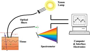
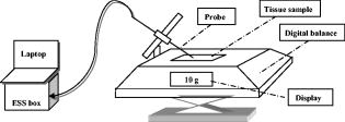
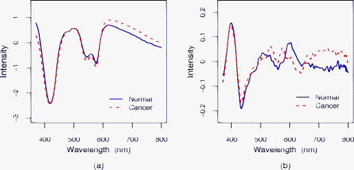
1.IntroductionThe incidence of esophageal adenocarcinoma has increased dramatically since the 1970s, and it is now the fifth commonest cause of cancer death in the UK. The five-year survival rate for this cancer is less than 10%.1, 2 Barrett’s esophagus (BE) is a premalignant condition in which the normal squamous epithelium of the esophagus is replaced by metaplastic columnar epithelium,3 increasing the risk of developing adenocarcinoma by 30 to 125 times4, 5, 6, 7 when compared to the general population. Systematic endoscopic surveillance of BE has been shown to detect esophageal adenocarcinoma at an early and curable stage.8 High-grade dysplasia (HGD) is the current most robust predictor of future cancer risk in patients with BE, with around 50% progressing to adenocarcinoma at five years if it is not treated.9, 10 Endoscopic surveillance relies on regularly spaced, but essentially random, biopsies being taken from the four quadrants of the Barrett’s segment every . It is time-consuming and labor intensive and has a low detection rate for HGD, even when abnormalities exist.11, 12 The challenge for clinicians and scientists is to develop new technologies for detecting patients at high risk of progression to cancer. Ideally, this would be accurate, easy to use, and inexpensive and would provide results rapidly, preferably without the need to remove tissue. Elastic scattering spectroscopy (ESS) is an in vivo optical point measurement, which, using an appropriate optical geometry, is sensitive to changes in the physical properties of tissue.13 The optical probe is passed through the working channel of an endoscope and is placed in direct contact with tissue. Short pulses of white light interrogate a small volume of superficial tissue approximately in diameter and deep. (See details in the following). Results are available within fractions of a second. Since the technology uses white light and produces a strong backscattered signal, components are inexpensive and the system is simple to manufacture. It is also safe, because only light in the range is used for illumination, with shorter-wavelength ultraviolet light being filtered out. Many of the features that pathologists look for in diagnosing HGD have also been shown to affect light scattering, including the nuclear:cytoplasmic ratio (in Monte Carlo modeling14); the cellular packing density;15 and the nuclear size.16 The nuclear chromatin content has also been shown to affect the spectra of both singly scattered light17, 18 and high angle scatter in ESS.19 ESS has been demonstrated clinically in a number of organ areas and disease types.20 The problem is how to maximize the discrimination between ESS spectra taken from high- and low-risk sites in order to accurately detect the patients at high future cancer risk. The difficulty is that the spectral differences between normal and abnormal tissue can be subtle compared to major sources of variation that are of little or no predictive value for the detection of cancer risk. In the clinical setting, it is extremely difficult even for experienced endoscopists to accurately control all aspects of ESS spectral acquisition, especially with respect to the angle and pressure of the optical probe in relation to the tissue with which it is in contact. It is known that pressure affects the spectra.21 Movement and other artifacts also occur and can affect the optical measurements collected. This is in part due to the proximity of the esophagus to the heart and lungs in the mediastinum, making it susceptible to coughing and breathing artifacts during endoscopy. If replicated spectra were to be taken in rapid succession from the same site (typically four in under one second) an appropriate statistical pretreatment method might be able to identify and reduce this intermeasurement variability, thus helping in the construction of an effective diagnostic model. In this work, we have employed a new statistical pretreatment method called error removal by orthogonal subtraction (EROS), which was introduced in an earlier paper.22 EROS uses replicated measurements to learn the structure of the measurement variability and an orthogonal projection matrix to subtract it mathematically from the spectra. 2.Materials and Methods2.1.Elastic Scattering Spectroscopy SystemThe ESS system consists of a pulsed xenon arc lamp, an optical probe, a spectrometer, and a computer to control these components and record the spectra. The arc lamp, spectrometer, and power supply are housed in a portable, briefcase-sized, unit to which the laptop computer is connected. Short pulses of white light from the xenon arc lamp (Perkin Elmer, Inc., Fremont, California) are directed through a flexible optical fiber, with the probe tip touching the tissue to be interrogated. Ultraviolet B and C light is filtered out to avoid risk to patients. A collection fiber ( diameter), with a fixed separation distance of (center-to-center) from an illumination fiber ( diameter), collects backscattered light from the upper layers of the tissue and conveys it to the spectrometer (S2000 Ocean Optics, Dunedin, Florida). The spectrometer outputs the spectrum to the computer for recording and further analysis (Fig. 1 ). The fiber assembly is housed in a plastic sheath (outer diameter ), which can pass into the esophagus via the biopsy channel of a standard endoscope. Collection and recording of a single spectrum takes approximately . 2.2.Laboratory Experiment2.2.1.Purpose of experimentTwo potential sources of significant measurement variability when collecting data in vivo are variations in the pressure of the probe on the tissue and in the angle at which the probe is held to the tissue.23, 24 These factors are difficult to control during measurement under typical clinical conditions. In the experiment reported here, they were deliberately varied in a controlled fashion in order to investigate their effects on the spectra. 2.2.2.Materials, instruments, and methodsTwo different types of tissues, squamous-cell-lined pig esophagus and columnar-cell-lined pig stomach, were resected, using a portion of approximately of each tissue, extended on a small piece of cork and fixed with pins. This preparation was placed on an electronic balance, as illustrated in Fig. 2 . All measurements were carried out with a (outer diameter) optical biopsy probe, which contains both the illuminating and collecting fibers. As described earlier, these fibers had a center-to-center separation of .25 Data were collected at six random sites for each tissue. At each site, 10 replicate measurements were taken under the conditions of all possible combinations of four pressures ( , , , ) and four angles to the vertical ( , , , ). Thus, the total number of spectra measured for each tissue was 960. To achieve the conditions, the probe was fixed to a micromanipulator at the desired angle and pushed downward until the balance gave the desired reading. The force measured by the balance was converted to a pressure using an approximate contact area of for the probe tip. 2.3.In Vivo Spectral AcquisitionThis study was approved by the joint University College London/University College London Hospitals (UCLH) Ethics Committee. During routine endoscopy, optical measurements were taken, followed immediately by biopsy from the same sites. A total of 152 matched optical and histological biopsy sites were collected from 81 patients referred to our tertiary referral center between 2000 and 2003 for the management of high-grade dysplasia (HGD) or early cancer in BE. Informed consent was obtained from all patients prior to their participation in the study. Before any tissue spectra were taken, a white reference spectrum was recorded from the spectrally flat diffuse reflector (Spectralon, Labsphere, Inc., North Sutton, New Hampshire). This provided calibration of the overall system response, to account for spectral variations in the light source, spectrometer, fiber transmission, and fiber coupling. ESS spectral data used in our analysis is the ratio of the spectral intensity of backscattered light from the tissue to that of the standard reference spectrum from Spectralon. Each spectrum was made up of from the detector, spanning the wavelength range , although the actual spectral resolution was about . Spectra were taken from one to three sites per patient, with a median of four spectra from each site (mean 3.3). Of the 152 matched optical and histological biopsies (corresponding to 506 spectra), 122 (corresponding to 413 spectra) were from low-grade dysplasia or no dysplasia (low risk) and 30 (corresponding to 93 spectra) were from high-grade dysplasia or cancer (high risk). Each biopsy was assessed and assigned as either high or low risk by three pathologists, who met to generate a consensus in cases of disagreement. This data set was used to train classification rules, as described in Sec. 2.4. A new data set with a total of 68 matched optical and histological biopsies (corresponding to 276 spectra) was collected from another 20 patients. These measurements were made later in time than those in the training set and were not looked at until after the diagnostic models had been selected and trained. The set included 50 biopsies (corresponding to 202 spectra) from low-grade dysplasia or no dysplasia (low risk) and 18 biopsies (corresponding to 74 spectra) from high-grade dysplasia or cancer (high risk). This data set was used for prospective prediction, as described in Sec. 2.4. All raw spectra were visually examined for any obvious outliers caused by acquisition errors, poor contact of the optical probe with the tissue, dirt/blood on the probe tip, or other artifacts. These spectra, from 16 biopsy sites, were excluded from subsequent analysis. 2.4.Statistical AnalysisStandard data preprocessing was carried out on the spectra to improve signal quality.25, 26 The spectra were first smoothed using the Savitzky-Golay method,27 spanning a 7-point window below and spanning a 20-point window above , where noise was greater. To speed subsequent manipulation, the smoothed data were then reduced from the , given the spectrometer resolution of , by taking alternate points only. To remove the regions of the spectra with low signal-to-noise ratios arising from the lower system response, only the wavelengths between 370 and , with 637 points, were used in the analysis. Using the standard normal variate (SNV)28 method, the spectra were then normalized by setting the mean intensity of each spectrum to zero and the variance to one. To study the spectra from the laboratory experiment, a principal component analysis (PCA) based on the pooled within-site covariance matrix22 was carried out separately for each type of tissue. The loadings for the first few principal components describe how pressure and angle affect the experimental spectra. The results for the two types of tissue being similar, the within-site covariance matrix was then pooled over all 12 sites, and a further PCA carried out. A PCA was also carried out on the pooled within-site covariance matrix of the in vivo spectra. The loadings for the first few principal components from this analysis describe the variability in in vivo replicate measurements. The two sets of loadings, for experimental and in vivo spectra, were compared. A new spectral pretreatment method, error reduction by orthogonal subtraction (EROS), described in detail elsewhere,22 was applied to the in vivo spectra. EROS deals with problems related to measurement variability. It uses replicated measurements from what is nominally the same site to model the structure of the measurement variability, and then subtracts this variability from the spectra. The modeling involves a PCA of the pooled within-site covariance matrix of the in vivo spectra, as described earlier. The result of this is a set of principal component loadings that describe the measurement variability. The subtraction is carried out by projecting the spectra onto the space orthogonal to that spanned by a chosen number, , of these principal components. This is equivalent to subtracting from each spectrum the best fitting (in a least-squares sense) linear combination of the selected principal component loadings. Using the in vivo training data set described in Sec. 2.3, classification rules were derived from both the original spectra and the EROS pretreated spectra using principal component discriminant analysis (PCDA): an initial PCA on the spectra, followed by linear discriminant analysis (LDA) on the first PC scores.22 EROS and PCDA were carried out for a grid of values of and , with ranging from 0 (no dimensions subtracted) to 7 and from 5 to 30. Leave-out-one-site cross-validation22 trained the algorithm, i.e., carried out the EROS pretreatment followed by the PCA and the LDA, on all the data except one site, and the excluded site was then predicted. This was used to assess the performance of the classification, as measured by sensitivity, specificity and AUC, the area under a receiver operating characteristic (ROC) curve showing the sensitivity versus the false positive rate (1-specificity), generated by varying the threshold canonical score. In this per-site analysis, if any one of the spectra from a particular biopsy site was classified as a spectrum from a high-risk site, the whole biopsy site was regarded as a high-risk one. To test the robustness of the models, predictions were made for the separate Barrett’s test set described in Sec. 2.3. The same spectral pretreatment procedures were implemented on these data as mentioned earlier, followed by an application of the classification rules derived from the training data described in Sec. 2.3 using cutoffs also learned from the training data. All the computations and analyses were performed using the R statistical language (www.r-project.org). R is a free software environment for statistical computing and graphics. 3.Results3.1.Measurement VariabilityExamination of the laboratory data, where pressure and angle have been deliberately varied, and comparison of these data with in vivo spectra showed that these factors do affect the spectra and are probably responsible for much of the variability in the in vivo spectra. That pressure and angle affect the spectra is evident from Fig. 3, with a clear ordering of the mean spectra for the squamous tissue being visible as each factor is varied. The picture is similar for the columnar tissue. It is not surprising that these factors affect the spectra, for they will affect the contact of the probe and the density of the tissue beneath it. To demonstrate the similarity between the spectral variability in the laboratory and in vivo situations, the first three principal component loadings, based on the pooled within-site covariance matrix, are plotted in Fig. 4 for both the experimental data and the in vivo Barrett’s data. For each principal component, the experimental and in vivo loadings are similar. The first component, almost a linear trend with wavelength, and the second, resembling an inverted mean spectrum, suggest that variations in baseline and scale are dominant in both systems. The third component is harder to interpret, but still shows a broadly similar shape in the two cases. For the experimental data, the pooled within-sample covariance captures the variation caused by pressure and angle under controlled laboratory conditions. For the in vivo Barrett’s data, it describes the variability between replicate measurements. The similarity in the loadings supports the contention that much of the variability in the in vivo replicate measurements comes from differences in pressure and/or angle. Fig. 3Spectral pattern of squamous tissue. (a) Solid black, solid gray, dotted black, and dotted gray lines: Mean spectra measured under the condition of different pressure levels , , , , respectively. (Results are combined for all angles.) (b) Solid black, solid gray, dotted black, and dotted gray lines: Mean intensity of spectra measured under the condition of different angle levels , , , , respectively. (Results are combined for all pressures.)  3.2.Effect of EROS Pretreatment on In Vivo SpectraThe two panels of Fig. 5 show the mean spectra for low- and high-risk sites, before and after pretreatment with EROS, in which dimensions were removed. Differences between the means are much more evident in the right-hand panel, after pretreatment. What cannot be seen from the figure, because the spectra have been rescaled, is that the pretreatment has removed 96.6% of the variability in the original spectra. 3.3.Effect of EROS on the Construction of a Diagnostic RuleThe in vivo data were used to construct diagnostic rules for the detection of HGD or cancer both with and without the use of EROS, fixing the sensitivity at 90% in each case. Examination of plots that show how each wavelength contributes to the discrimination revealed a reduction in noise and an improvement in interpretability when EROS was used. Table 1 shows the leave-out-one-site cross-validation results for detection of HGD or cancer for various combinations of , the number of dimensions removed by the EROS pretreatment, and , the number of principal components used in the construction of the diagnostic rule. In deriving the rule, the “cutoff” canonical score between the high-risk and low-risk sites was chosen to give a sensitivity of 90% each time. This high sensitivity comes at the expense of specificity, but it was felt to be a greater omission to potentially “miss” patients at high risk than to have to collect a few additional biopsies (due to ESS false positives). In the clinical model we envision, conventional biopsies would be taken only if the ESS spectrum was indicative of dysplasia or cancer. Table 1Results of leave-out-one-site cross-validation on Barrett’s data set using various combinations of k (number of dimensions removed by EROS pretreatment) and q (number of PC scores used in the LDA). All the diagnostic rules have a sensitivity of 90%.
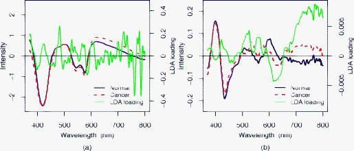
Without pretreatment by EROS ( in Table 1), the choice gives the best results with sensitivity, specificity, and AUC of 90%, 67%, and 0.82, respectively, comparable with those reported in Ref. 25 for a related but slightly different data set (92%, 60%, 0.85). When at least dimensions are removed by EROS, the number of components required to construct a good diagnostic rule falls substantially. In particular, the combination , gives the best results, with sensitivity, specificity, and AUC of 90%, 82%, and 0.86, respectively. Figure 6 compares the loadings for the LDA discriminant functions using , (no EROS) in the left panel and , in the right panel. These loadings show the contribution at each wavelength to the linear diagnostic rule, and thus permit interpretation of its spectral basis. With EROS, and thus using many fewer factors in the classification model, the loading vector is much less noisy and can be related much more easily to features in the spectra. In the right-hand panel of Fig. 6, the most obvious feature is a large positive LDA loading in the region of and peaking at around , corresponding to clear differences between the mean spectra. The peak at is consistent with a lowered oxygen saturation of haemoglobin in dysplastic tissue, as has been noted by various research groups.29, 30 Two peaks in the LDA loading around 540 and may be due to absorption dips of at 542 and in the spectra of high-risk cancer due to increased Hb presence. It is known that cancers and precancerous tissues are characterized by increased microvascular volume, and hence increased blood content.31 3.4.Prospective PredictionThe two best models, those using , (no EROS) and , (EROS), were applied to the independent test set. The EROS model gave better prediction results with sensitivity of 83% and specificity of 84%, compared with a sensitivity of 78% and specificity of 66% without EROS. Both models showed some loss of sensitivity compared with the 90% on the training set, but the specificity was maintained in both cases, which was the advantage of EROS. 4.DiscussionThe importance of variations in pressure and angle at the time of spectral measurement has been confirmed by a designed experiment. Pretreatment with EROS was used to characterize and remove this variability from in vivo spectral data before developing a diagnostic rule. In this case, the diagnostic rule employed PCA followed by LDA, but it would be perfectly possible to combine EROS with other approaches to classification. The resulting simplification of the spectral data has two benefits. The removal of noise should lead to more robust predictions, as demonstrated on the independent test set. This is crucial for real-time clinical diagnostic application. In addition, simpler and smoother loadings for the classification rule will facilitate interpretation of the spectral basis for the rule. This interpretation of the LDA loading will be further developed in future work. In conclusion, this work provides a better understanding of how spectral changes are generated by scattering and absorption and how they contributed to classification. EROS allows the development of a more accurate and robust diagnostic algorithm system in which ESS acts as a straightforward, reliable, and valuable technique for the rapid and accurate early detection of cancer risk in Barrett’s esophagus. AcknowledgmentsThe authors are grateful to the Peacock Trust, the National Cancer Institute Network for Translational Research into Optical Imaging (NTROI) of NIH, Experimental Cancer Medicine Centre (ECMC), and Comprehensive Biomedical Research Centre (CBRC) for their support of this work at University College London (UCL). ReferencesA. Newnham, M. J. Quinn, P. Babb, J. Y. Kang, and A. Majeed,
“Trends in the subsite and morphology of oesophageal and gastric cancer in England and Wales 1971–1998,”
Aliment Pharmacol. Ther., 17
(5), 665
–676
(2003). https://doi.org/10.1046/j.1365-2036.2003.01521.x 0269-2813 Google Scholar
CancerStats Monograph 2004, Cancer Research UK, London
(2004). Google Scholar
R. W. Phillips and R. K. Wong,
“Barrett’s esophagus. Natural history, incidence, etiology, and complications,”
Gastroenterol. Clin. North Am., 20
(4), 791
–816
(1991). 0889-8553 Google Scholar
A. J. Cameron, B. J. Ott, and W. S. Payne,
“The incidence of adenocarcinoma in columnar-lined (Barrett’s) esophagus,”
N. Engl. J. Med., 313
(14), 857
–859
(1985). 0028-4793 Google Scholar
W. A. Williamson, F. H. Ellis Jr., S. P. Gibb, D. M. Shahian, H. T. Aretz, G. J. Heatley, E. Watkins Jr.,
“Barrett’s esophagus. Prevalence and incidence of adenocarcinoma,”
Arch. Intern Med., 151
(11), 2212
–2216
(1991). https://doi.org/10.1001/archinte.151.11.2212 0003-9926 Google Scholar
C. S. Robertson, J. F. Mayberry, D. A. Nicholson, P. D. James, and M. Atkinson,
“Value of endoscopic surveillance in the detection of neoplastic change in Barrett’s oesophagus,”
Br. J. Surg., 75
(8), 760
–763
(1988). https://doi.org/10.1002/bjs.1800750813 0007-1323 Google Scholar
W. Hameeteman, G. N. Tytgat, H. J. Houthoff, and J. G. van den Tweel,
“Barrett’s esophagus: development of dysplasia and adenocarcinoma,”
Gastroenterology, 96
(5), 1249
–1256
(1989). 0016-5085 Google Scholar
D. S. Levine, R. C. Haggitt, P. L. Blount, P. S. Rabinovitch, V. W. Rusch, and B. J. Reid,
“An endoscopic biopsy protocol can differentiate high-grade dysplasia from early adenocarcinoma in Barrett’s esophagus,”
Gastroenterology, 105
(1), 40
–50
(1993). 0016-5085 Google Scholar
P. S. Rabinovitch, G. Longton, P. L. Blount, D. S. Levine, and B. J. Reid,
“Predictors of progression in Barrett’s esophagus III: baseline flow cytometric variables,”
Am. J. Gastroenterol., 96
(11), 3071
–3083
(2001). https://doi.org/10.1111/j.1572-0241.2001.05261.x 0002-9270 Google Scholar
V. K. Sharma, K. K. Wang, B. F. Overholt, C. J. Lightdale, M. B. Fennerty, P. J. Dean, D. K. Pleskow, R. Chuttani, A. Reymunde, N. Santiago, K. J. Chang, M. B. Kimmey, and D. E. Fleischer,
“Balloon-based, circumferential, endoscopic radiofrequency ablation of Barrett’s esophagus: follow-up of 100 patients,”
Gastrointest. Endosc., 65
(2), 185
–195
(2007). https://doi.org/10.1016/j.gie.2006.09.033 0016-5107 Google Scholar
J. W. van Sandick, J. J. van Lanschot, B. W. Kuiken, G. N. Tytgat, G. J. Offerhaus, and H. Obertop,
“Impact of endoscopic biopsy surveillance of Barrett’s oesophagus on pathological stage and clinical outcome of Barrett’s carcinoma,”
Gut, 43
(2), 216
–222
(1998). 0017-5749 Google Scholar
H. Messmann, R. Knuchel, W. Baumler, A. Holstege, and J. Scholmerich,
“Endoscopic fluorescence detection of dysplasia in patients with Barrett’s esophagus, ulcerative colitis, or adenomatous polyps after 5-aminolevulinic acid-induced protoporphyrin IX sensitization,”
Gastrointest. Endosc., 49
(1), 97
–101
(1999). https://doi.org/10.1016/S0016-5107(99)70453-0 0016-5107 Google Scholar
L. B. Lovat and S. G. Bown,
“Elastic scattering spectroscopy for detection of dysplasia in Barrett’s esophagus,”
Gastroenterol. Clin. North Am., 14
(3), 507
–517
(2004). https://doi.org/10.1016/j.giec.2004.03.006 0889-8553 Google Scholar
R. Drezek, A. Dunn, and R. Richards-Kortum,
“Light scattering from cells: finite-difference time-domain simulations and goniometric measurements,”
Appl. Opt., 38
(16), 3651
–3661
(1999). https://doi.org/10.1364/AO.38.003651 0003-6935 Google Scholar
M. B. Wallace, L. T. Perelman, V. Backman, J. M. Crawford, M. Fitzmaurice, M. Seiler, K. Badizadegan, S. J. Shields, I. Itzkan, R. R. Dasari, J. Van Dam, and M. S. Feld,
“Endoscopic detection of dysplasia in patients with Barrett’s esophagus using light-scattering spectroscopy,”
Gastroenterology, 119
(3), 677
–682
(2000). https://doi.org/10.1053/gast.2000.16511 0016-5085 Google Scholar
G. Zonios, L. T. Perelman, V. M. Backman, R. Manoharan, M. Fitzmaurice, J. Van Dam, and M. S. Feld,
“Diffuse reflectance spectroscopy of human adenomatous colon polyps in vivo,”
Appl. Opt., 38
(31), 6628
–6637
(1999). https://doi.org/10.1364/AO.38.006628 0003-6935 Google Scholar
R. S. Gurjar, V. Backman, L. T. Perelman, I. Georgakoudi, K. Badizadegan, I. Itzkan, R. R. Dasari, and M. S. Feld,
“Imaging human epithelial properties with polarized light-scattering spectroscopy,”
Nat. Med., 7
(11), 1245
–1248
(2001). https://doi.org/10.1038/nm1101-1245 1078-8956 Google Scholar
V. Backman, M. B. Wallace, L. T. Perelman, J. T. Arendt, R. Gurjar, M. G. Müller, Q. Zhang, G. Zonios, E. Kline, T. McGillican, S. Shapshay, T. Valdez, K. Badizadegan, J. M. Crawford, M. Fitzmaurice, S. Kabani, H. S. Levin, M. Seiler, R. R. Dasari, I. Itzkan, J. Van Dam, and M. S. Feld,
“Detection of preinvasive cancer cells,”
Nature, 406
(6791), 35
–36
(2000). https://doi.org/10.1038/35017638 0028-0836 Google Scholar
J. R. Mourant, M. Canpolat, C. Brocker, O. Esponda-Ramos, T. Johnson, A. Matanock, K. Stetter, and J. P. Freyer,
“Light scattering from cells: the contribution of the nucleus and the effects of proliferative status,”
J. Biomed. Opt., 5
(2), 131
–137
(2000). https://doi.org/10.1117/1.429979 1083-3668 Google Scholar
I. J. Bigio and S. G. Bown,
“Spectroscopic sensing of cancer and cancer chemotherapy, current status of translational research,”
Cancer Biol. Therapy, 3
(3), 259
–267
(2004). Google Scholar
R. Reif, M. S. Amorosino, K. W. Calabro, O. Aamar, S. K. Singh, and I. J. Bigio,
“Analysis of changes in reflectance measurements on biological tissues subjected to different probe pressures,”
J. Biomed. Opt., 13 010502-1
–3
(2008). https://doi.org/10.1117/1.2870115 1083-3668 Google Scholar
Y. Zhu, T. Fearn, D. Samuel, A. Dhar, O. Hameed, S. G. Bown, and L. B. Lovat,
“Error removal by orthogonal subtraction (EROS): a customized pretreatment for spectroscopic data,”
J. Chemom., 22
(2), 130
–134
(2008). https://doi.org/10.1002/cem.1117 0886-9383 Google Scholar
C. A. Gonzalez-Correa, B. H. Brown, R. H. Smallwood, N. Kalia, C. J. Stoddard, T. J. Stephenson, S. J. Haggie, D. N. Slater, and K. D. Bardhan,
“Assessing the conditions for in vivo electrical virtual biopsies in Barrett’s oesophagus,”
Med. Biol. Eng. Comput., 38
(4), 373
–376
(2000). https://doi.org/10.1007/BF02345004 0140-0118 Google Scholar
C. A. Gonzalez-Correa, B. H. Brown, R. H. Smallwood, D. C. Walker, and K. D. Bardhan,
“Electrical bioimpedance readings increase with higher pressure applied to the measuring probe,”
Physiol. Meas, 26
(2), S39
–S47
(2005). https://doi.org/10.1088/0967-3334/26/2/004 0967-3334 Google Scholar
L. B. Lovat, K. S. Johnson, G. D. Mackenzie, B. R. Clark, M. R. Novelli, S. Davies, M. O’Donovan, C. Selvasekar, S. M. Thorpe, D. Pickard, R. Fitzgerald, T. Fearn, I. Bigio, and S. G. Bown,
“Elastic scattering spectroscopy accurately detects high grade dysplasia and cancer in Barrett’s oesophagus,”
Gut, 55
(8), 1078
–1083
(2006). https://doi.org/10.1136/gut.2005.081497 0017-5749 Google Scholar
T. Næs, T. Isaksson, T. Fearn, and T. Davies, A User-Friendly Guide to Multivariate Calibration and Classification, NIR Publications, Chichester, UK
(2002). Google Scholar
A. Savitzky and M. J. E. Golay,
“Smoothing and differentiation of data by simplified least-squares procedures,”
Anal. Chem., 36
(8), 1627
–1639
(1964). https://doi.org/10.1021/ac60214a047 0003-2700 Google Scholar
R. J. Barnes, M. S. Dhanoa, and S. J. Lister,
“Standard normal variate transformation and de-trending of near-infrared diffuse reflectance spectra,”
Appl. Spectrosc., 43
(5), 772
–777
(1989). https://doi.org/10.1366/0003702894202201 0003-7028 Google Scholar
D. L. Conover, B. M. Fenton, T. H. Foster, and E. L. Hull,
“An evaluation of near infrared spectroscopy and cryospectrophotometry estimates of haemoglobin oxygen saturation in a rodent mammary tumour model,”
Phys. Med. Biol., 45
(9), 2685
–2700
(2000). https://doi.org/10.1088/0031-9155/45/9/318 0031-9155 Google Scholar
N. Shah, A. E. Cerussi, D. Jakubowski, D. Hsiang, J. Butler, and B. J. Tromberg,
“The role of diffuse optical spectroscopy in the clinical management of breast cancer,”
Dis. Markers, 19
(2–3), 95
–105
(2004). 0278-0240 Google Scholar
R. K. Jain,
“Determinants of tumor blood flow: a review,”
Cancer Res., 48
(10), 2641
–2658
(1988). 0008-5472 Google Scholar
|
||||||||||||||||||||||||||||||||||||||||||||||||||||||||||||||||||||||||||||||||||||||