1.

Introduction

Anisotropic transport of light has been observed in a number of random anisotropic opaque materials. Such transport occurs in aligned nematic liquid crystals,^{1, 2} human and animal tissue (including bone,³ muscle,⁴ teeth,⁵ skin,⁶ arterial walls,⁷ blood cells under shear,⁸) and porous semiconductors,^{9, 10} to name a few. Given the technological and medical importance of such materials, understanding the fundamental principles of diffuse anisotropic light transport as well as finding appropriate approximations for such transport is essential.

However, these materials do not necessarily conform easily to controlled experiments and analysis. For example, observing anisotropic diffusion in a nematic liquid crystal requires a relatively large cell with a perfectly aligned sample.^{1, 2} Furthermore, in such a system, the anisotropy is relatively weak compared to, for example, fibrous materials and porous semiconductors. ^{9, 10, 11} Human tissue, while fascinating and important to study, has a complex microstructure with inhomogeneities that may be difficult to approximate theoretically. Therefore, while it is vital to understand anisotropic diffusion in human tissue, this material may not be the most ideal for testing theories of anisotropic diffusion. Other materials, such as porous semiconductors, are difficult to cleave smoothly, making access to various orientations of the anisotropy challenging. For these reasons, model (phantom) systems for studying anisotropic transport are useful.

For such model systems to be useful for theoretical modeling, they should be homogeneous and easily manipulated. The microscopic structure (the structure at the scale of light wavelengths) should be well-defined and measurable. Such characteristics allow detailed tests of theoretical predictions of anisotropic transport at both the macroscopic and microscopic scale.

One anisotropic model sample has been previously produced, a randomly positioned collection of parallel wax fibers in a solid cube of resin.¹² In this sample, cylindrical fibers of $1.5\mathrm{mm}$ diameter were extended through a block of epoxy with dimensions on the order of $5\text{to}15\mathrm{cm}$ . Thus, it was composed of many small isotropic scatterers and few long, anisotropic structures with diameters several orders of magnitude larger than the wavelength of light. This sample proved useful for testing theories of time-resolved propagation in anisotropic materials. However, in this sample, the anisotropic scatterers themselves (the fibers) are as large as the sample. This raises the possibility of long-range light guiding rather than diffusion, as noted by the authors.¹² This sample is not conducive to the study of oblique cross sections with respect to the fiber orientation, since such cleaves would also create unusual surface scatterers.

Theoretically, the problem of anisotropic optical diffusion has been modeled analytically using anisotropic random walk models¹³ and radiative transfer approaches, ^{14, 15, 16} and numerically using Monte Carlo simulations.⁷ A solution to the diffusion equation for an anisotropic diffusion tensor with oblique orientation with respect to the sample surface was recently derived by Dudko and Weiss.¹⁷

There have been several points of contention in the theoretical discussion of anisotropic diffuse light. For example, it has been questioned whether the diffusion constant ratio itself can be measured by any static measurement, it being a dynamic quantity.² Recently, we have shown that the anisotropic diffusion model is experimentally applicable for several sample orientations,¹¹ although it has yet to be tested with an oblique orientation of the diffusion constant tensor. There is only one demonstration of theoretically connecting the microstructure of an anisotropic system to the diffusion tensor.¹⁴ One recent paper has called this type of analysis into question, with the proposition that only Monte Carlo simulations of the radiative transport equations provide useful models of the connection between microscopic structure and anisotropic multiple scattering.¹⁸ Thus, it would be useful to test this type of analysis for a wide variety of well-defined sample geometries.

In this article, we present a collection of new experimental anisotropic opaque systems along with models for light propagation derived from the scattering properties of individual scatterers. The materials we have created have high optical anisotropies, have relatively small anisotropic scatters (on the order of wavelengths to hundreds of wavelengths), and are easily cleaved in any direction to allow for arbitrary orientation of the scatterers. The scatterers in these systems may be approximated by simple geometrical structures: cylinders, planes, and ellipsoids. We are able to model the transmission of light in these materials using diffusion theory. We have also tested the model of Dudko and Weiss¹⁷ to model light propagation for one sample with oblique orientation of the diffusion tensor. Last, we use microscopic models to analytically derive a diffusion constant for two of these systems and suggest methods for applying these equations to other systems of interest. Our theoretical predictions from these models for the diffusion constant are consistent with the experimental measurements on the model systems, thus supporting our approach.

2.

Experiment

2.1.

Sample Fabrication

The anisotropic model systems were chosen taking into account several important considerations. The sample should be statistically anisotropic with a substantial degree of randomness to produce opaqueness when viewed from all directions. The sample should be uniform in structure to ensure reproducible measurements on separate parts of the sample and to support the assumption of position-independent parameters. The samples should be easy to obtain for use by experimentalists from a range of disciplines and backgrounds.

There are several other useful criteria. It is desirable for the structure to be controllable so that the anisotropy can be varied. This can be achieved in the case of plastic samples by stretching the sample. It is useful to have available samples with different internal geometry, for studying the relationship between microscopic geometry and macroscopic optical properties. Last, it is useful to have samples that can be fabricated with different orientations of the diffusion constant tensor. This can be achieved by having samples that are easily cleaved along different axes without disturbing the integral structure of the sample.

We present here three categories of samples that meet these criteria: (1) fibrous samples, for which we chose a porous fiber slab and Teflon tape; (2) stretched plastic frit; and (3) stretched foam. The internal geometry of these structures can be approximated as statistically aligned cylinders, ellipsoids, and planes, respectively.

2.1.1.

Fibrous samples

A porous fiber slab composed of pressed polyester/polyethylene (PET/PE) fibers was obtained from Porex Corporation. This material has been previously studied by us.¹¹ This material is used in exacting filter applications and comes in a variety of densities and fiber diameters. For our measurements, we chose fiber diameters of $10\mu \mathrm{m}$ and a density of $0.37\mathrm{g}∕{\mathrm{cm}}^3$ , as listed by the manufacturer. This corresponds to a volume fraction of polymer of roughly 30% or less, depending on the exact density of the polymer (which was unknown). The relatively small fiber diameter meant that samples of several hundred microns were already optically thick. The density was optimal for strong scattering and easy slicing.

Scanning electron microscopy (SEM) photos of the samples reveal a statistically aligned fiber structure with a substantial degree of randomness (Fig. 1 ). The fibers are highly interconnected, reducing the probability of light guiding through a single fiber. SEM also reveals large air voids between the fibers, suggesting a low-volume fraction of fibers.

Fig. 1

SEM of the porous fiber sample. The scale bar is $1\mathrm{mm}$ . The inset shows the distribution of fiber orientations $P_c\left(\theta \right)$ , with a fit to an exponential function.

It is useful for our theoretical calculations to estimate the distribution of fiber orientations. This was achieved by randomly choosing locations on an SEM photo and measuring the orientation of the fiber by hand. The raw data was binned and the resulting function fitted to an exponential function:

Eq. 1

$n=A\exp (-\frac{\theta }{{\theta }_c})\propto P_c\left(\theta \right),$

where $n$ is the number of counts, and $A$ and ${\theta }_c$ are freely varied in the fit. $P_c\left(\theta \right)$ is the probability density of a randomly chosen fiber having a surface orientation $\theta$ . This data and fit is given in the inset of Fig. 1, yielding ${\theta }_c=(18\pm 3)\mathrm{deg}$ . The function itself was chosen mainly for its simplicity, as it will be used in the following theoretical calculations.

The porous fiber slabs can be easily sliced along any axis using a razor blade. For the purposes of our experiments, we sliced the sample at an angle $(43\pm 2)\mathrm{deg}$ with respect to the surface. As seen from the optical micrographs in Fig. 2, the sliced samples retain a uniform fiber distribution, and the fibers remain well aligned at the surfaces.

Fig. 2

Optical micrograph of the cleaved porous fiber sample. The orientation of the fibers is $(43\pm 2)\mathrm{deg}$ with respect to the horizontal surface. The quality of the surface is not disturbed by the cleave, allowing accurate measurements of anisotropic diffusion with an oblique orientation of the diffusion constant tensor.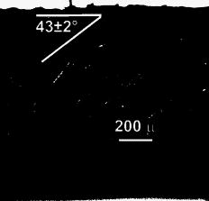

A second fibrous structure, Teflon tape, was also studied. The Teflon tape can be stretched to produce different degrees of physical anisotropy in the structure. The specific changes in structure associated with stretching have been studied in connection with superhydrophobicity.¹⁹ An SEM of the Teflon tape used in this study is given in Fig. 3 . As seen in the figure, the fibers are highly aligned. However, as will be demonstrated, even a simple material such as Teflon tape has unusual secondary structural characteristics that strongly influence the anisotropy in the light propagation.

Fig. 3

SEM of Teflon tape. The scale bar is $1\mu \mathrm{m}$ . The fibers are highly aligned. The fibrous regions occur in clusters with solid regions of Teflon between. The edges of solid regions can be seen in the top right and lower left of the photo.

2.1.2.

Stretched plastic frit

A second type of plastic sample was synthesized from porous plastic frit samples. These materials are used for filtration and are readily available from Porex Corporation in a variety of pore sizes ranging from several to hundreds of microns. For our experiment, we chose the most strongly scattering of these samples (Porex Corp., PE sheet, XS-7744 pore size $7\text{to}12\text{microns}$ ). The sheets are available in a variety of thicknesses. For most of our experiments, we used sheets that were $3\mathrm{mm}$ thick. Similar to the porous fiber system, these samples could be easily sliced along any axis with a scalpel. The plastic frit sheets are optically and physically isotropic [Fig. 4a ]. However, stretching the sheets yields optically anisotropic materials.

Fig. 4

Optical micrographs of plastic frit (a) after stretching at room temperature (b) after stretching to twice the length at $160°\mathrm{C}$ , and (c) after stretching to twice the length at $170°\mathrm{C}$ . An illustration of the slidable clamps is shown at the top of the figure. As seen in the images, stretching at room temperature yields no distortion of the particles, stretching at $160°\mathrm{C}$ yields distorted particles, and stretching at $170°\mathrm{C}$ yields again little distortion of the particles with narrow filaments between. The scale bar at the lower right, which applies to all three images, is $20\mu \mathrm{m}$ .

This stretching was attempted at four temperatures: $20°\mathrm{C}$ , $130°\mathrm{C}$ , $160°\mathrm{C}$ , and $170°\mathrm{C}$ . The sample was clamped on both ends, with the clamps attached to rail-bars, allowing for the distance between the clamps to be easily adjusted by hand (Fig. 3 top). The entire holder and sample was placed in a preheated oven for $15\min$ until the material was soft and then quickly (within a few seconds) stretched by hand to twice its length outside the oven.

Optical micrographs of the resulting stretched samples show three different structures (Fig. 4). At room temperature, stretching did not distort the shape of the particles at all, but simply rearranged the inter particle contacts. For these samples, we measured no optical anisotropy, which is understandable since only the density of particles was changed. At high temperatures $(170°\mathrm{C})$ , the particles form narrow connecting necks between the spheres. This also produces immeasurably small optical anisotropies. Despite the presence of the aligned anisotropic necks, we suggest that they are more weakly scattering than the undeformed (isotropic) spheres, i.e., the isotropic scatterers contribute overwhelmingly to the scattering. At $160°\mathrm{C}$ , the spheres themselves are deformed into more elliptical forms. In this case, the strongest scatterers are themselves deformed, resulting in anisotropic diffusion, as will be shown in the following.

2.1.3.

Plastic foam

Plastic foam samples were obtained from Reticel Technical Foams (LD 24, white). These are closed-cell foams of low-density polyethylene with cell sizes ranging from $100\text{to}400\text{microns}$ [Fig. 5a ]. The foams are flexible enough to be stretched at room temperature.

Fig. 5

Optical micrographs of plastic foam (a) before and (b) after stretching. The scale bar in (a) is $300\mu \mathrm{m}$ , which applies to both images. For demonstrating the change in structure, several single cells have been outlined in black both before and after stretching (different cells before and after stretching). The plot in the bottom left inset gives a histogram of the orientation of each linear cross section of the cell facets, weighted by the length of the cross section in pixels. This allows an estimation of the statistical probability per unit volume of finding a plane with orientation $\theta$ . The resulting distribution is linear, with an intercept of zero near $\theta =\pi ∕2$ .

The foams were stretched with the same setup used for stretching the plastic frit [Fig. 4a] at room temperature. Since the foams retain their elasticity at room temperature, the ends need to be fixed in place once the material is stretched. This was achieved by leaving the foam sample in the rail-bar holder during measurements. This method allowed the foams to be stretched to up to $1.5\times$ their length and produces a uniform distortion in the cell structure, as seen in Fig. 5.

Stretching the foam beyond $1.5\times$ leads to breakage, while stretching at increased temperatures distorted the homogeneity of the foam. Due to the elasticity of the sample, the stretched foams have the disadvantage that they could not be sliced or probed along oblique axes. Furthermore, since the clamps needed to remain fixed to the foam, the sides perpendicular to the stretch direction could not be accessed for optical measurements. However, the planar geometry of the foams offers an interesting structure for theoretical modeling.

As for the fibers, a numerical estimate of the microstructure is useful for the application of theoretical models. To this end, we have estimated the probability distribution for the linear cross sections as a function of angle $\theta$ with the stretch direction, weighted by the length of the facet cross section. This was carried out by measuring the orientation and length (in pixels) of all of the facet cross sections in a single optical micrograph. The length was used as a weight for each orientation. This distribution should be comparable to the probability per unit volume for finding a plane with an orientation $\theta$ . The result of this estimate is plotted in the inset of Fig. 5, showing a linear distribution with a zero intercept near $\theta =90\mathrm{deg}$ .

2.2.

Diffuse Transmission Measurements

To test the quality of these model systems and the applicability of the diffusion model, we have measured the diffuse transmission of light through all of these samples in a slab geometry. For all of the calculations, this slab is treated as a semi-infinite, with $w_1$ , $w_2⪢L$ , where $w_1$ , $w_2$ , are the two widths and the thickness of the sample, as shown in Fig. 6 .

Fig. 6

Illustration of the diffuse imaging geometry. Diffuse light is imaged at one side of the sample, the top side in the image, referred to as the image plane. The source beam is focused opposite to the image plane. The orientation of the elongated structure of the sample, suggested by the squiggles to the right of the image, is given by the orientation of $\widehat{s}$ and may be oblique with the surface, in which case it forms angle $\gamma$ with the $z$ axis. The image plane is parallel to the $x\text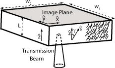{-}y$ plane.

The light source used was a supercontinuum broadband laser source (Fianium Femptopower 1060, $20\mathrm{MHz}$ ), attenuated with neutral density filters and with a bandpass filter (Thorlabs FB650-10), producing a collimated beam at $650\mathrm{nm}$ with a wide enough bandwidth ( $10\text{-}\mathrm{nm}$ FWHM) to eliminate speckle when imaging. For some measurements, a helium-neon laser was also used, which produced some speckle. For this laser, the speckle size was small enough that smoothing the image over a $10\text{-pixel}$ area on the camera substantially reduced the speckle without affecting the form of the average intensity distribution. The light escaping the image plane was imaged using a Peltier-cooled CCD (Andor iXon DV885JCS) equipped with a short range $(\approx 3\mathrm{cm})$ camera lens.

The source was focused with a numerical aperture of roughly 0.1. This kept the spot size small compared with $L$ , so as not to influence the diffuse pattern on the image plane, and the input solid angle of the beam small compared to $2\pi$ steradians, to limit the angular range of the input $k$ -vectors so that the focussed beam effectively enters the sample in one direction. The orientation of the incoming beam axis was perpendicular to the sample surface.

All of the samples have a uniaxial microscopic symmetry. This axis of symmetry could be aligned in various directions with respect to the slab geometry. Two of the samples, the porous fiber sample and the stretched plastic frit, allowed for the axis of symmetry to be at an oblique angle with respect to the image plane, providing a particularly interesting test of the diffusion model.

3.

Theoretical Solutions for Diffuse Transmission

The diffusion equation for anisotropic opaque media, assuming no absorption and a continuous wave source, is:

When the sample symmetry is aligned parallel or perpendicular to the sample surfaces, the diffusion tensor and the mean free path tensor are diagonal. This case has been experimentally and theoretically investigated previously.^{1, 9, 21, 22} $U$ can be derived by rescaling the coordinates by the respective diffusion tensors so as to reduce the anisotropic diffusion equation to Laplace’s equation. The solution to Laplace’s equation that satisfies the boundary condition requires the use of a series of image sources. The intensity distribution of light on the exiting side of the sample is given by Fick’s law, $I(x,y)=D_{zz}\partial U∕{\phantom{|}\partial z|}_{z=L}$ , yielding in this case:

Equation 2 can also be solved in the general case that $\mathbf{D}$ is not diagonal via a linear transformation of the coordinate system. This derivation has been carried out by Dudko and Weiss for the time-dependent diffusion equation with absorption.¹⁷ Ours is a specific case of that result. Therefore, we present here a brief overview of the derivation and refer the reader to Ref. 17 for details.

The solution requires a combination of coordinate rotations and rescalings. In the case of a uniaxial bulk material, one rotation is required to diagonalize the diffusion tensor. In this rotated reference frame, the $\widehat{z}$ axis is aligned with the symmetry axis $\widehat{s}$ of the bulk sample (see Fig. 6). This diagonalized matrix has the form:

The expression for ${\mathbf{r}}^{\prime }$ given in Eq. 6 is inserted into the isotropic version $(D_{xx}=D_{yy}=D_{zz})$ of Eq. 4, yielding the intensity profile for oblique orientation of the diffusion tensor. The resulting expression is somewhat complicated, although still analytic and readily calculated. This transformation and the resulting solution were calculated algebraically using MATLAB’s symbolic toolbox, yielding a function that could be pasted into MATLAB’s fitting routines. The resulting analytic expression for $I(x,y)$ , too long to be presented in this article, was simple enough to allow for rapid (order $10\mathrm{s}$ ) fitting of large $(>1\text{megabyte})$ two-dimensional (2-D) data sets in MATLAB. The results of this procedure were checked for consistency with those of Dudko and Weiss.¹⁷

4.

Results

The resulting iso-intensity lines for diffuse transmission were fit to the models for transmission. As seen in Fig. 7 and Fig. 8a, the foam, stretched plastic frit, Teflon tape, and plastic fiber all show excellent fits to Eq. 4 when the sample symmetry axes are parallel to the sample surface. In these fits, the position is stated in units of the sample thickness, leaving the anisotropy ratio $D_{yy}∕D_{xx}$ as the only fitting parameter. The fits yielded $D_{yy}∕D_{xx}=0.77\pm .02$ , $0.70\pm .02$ , $1.21\pm .02$ , and $0.28\pm 0.03$ for the plastic frit, foam, Teflon tape, and plastic fiber samples, respectively, where the $x$ axis is parallel the stretch direction of the frit and foam, and to the fiber orientation of the Teflon tape and plastic fiber. The orientation of the long axis of the iso-intensity ellipses, indicating the “fast axis” of diffusion, are parallel to the stretch direction of the frit and foam and parallel to the plastic fibers. By contrast, the fast axis of diffusion is perpendicular to the fiber orientation of the Teflon tape, as seen in Fig. 7c. The counterintuitive contrast between the plastic fiber and Teflon tape will be discussed in Sec. 5.

Fig. 7

Transmission data (rough iso-intensity lines) and fit to Eq. 4 (smooth iso-intensity lines) for (a) plastic frit, (b) foam, and (c) Teflon tape. All intensities are normalized by the peak intensity, and the separation in iso-intensity lines is 0.1. The innermost iso-intensity ellipse has the value 0.9. The model fits the data well for all three samples, demonstrating the effectiveness of the diffusion model for a variety of microstructures.

Fig. 8

Transmission data (rough iso-intensity lines) and fit (smooth iso-intensity lines) for two orientations of the fibers with respect to the sample surface, (a) parallel and (b) at an oblique $(43\pm 2)\mathrm{deg}$ angle with the surface for a plastic fiber sample, normalized to the peak intensity. The separation in iso-intensity lines is 0.1. The innermost iso-intensity ellipse has the value 0.9. The source is located at the zero positions, denoted by the crosshairs. In the top plot (a), Eq. 4 is used to fit the data. In the bottom plot (b), the derived equation for an oblique diffusion tensor is used to fit the data. The bottom of (a) is cut due to the limited imaging range of the camera.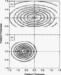

Fig. 8b shows the result for the plastic fiber sample with oblique orientation of the fibers. As for the stretched plastic frit, the orientation of the long axis of the ellipse is parallel to the fiber orientation. The source is located at the (0, 0) position of the crosshairs in the image. Thus, the light guiding due to scattering⁵ is apparent. The diffuse image has been shifted dramatically to the left due to the oblique orientation of the fibers.

The diffuse light for the obliquely oriented plastic fibers was matched to the analytic solution for Eq. 2 with the rotated reference frame described in Sec. 3. To test the consistency of the model, the parameters in the fit were limited to within previously determined ranges. The two free parameters were the orientation angle of the fibers $\gamma$ and the diffusion constant ratio. The resulting fit yields $B=0.23\pm 0.03$ and $\gamma =45\pm 2\mathrm{deg}$ . This is consistent with value of $B$ determined from the fit to Fig. 8a and the measured angle of $(43\pm 2)\mathrm{deg}$ giving good support for the diffusion model in the case of oblique orientation of the fibers.¹⁷

5.

Microscopic Modeling

In this section, we address the question, to what degree can a simple connection be made between the microscopic structure and macroscopic results? As seen from the experimental results, radically different microscopic structures may be modeled using the diffusion theory for optical transmission, including for oblique orientation of the diffusion tensor. From this modeling, we find some interesting contrasts in the resulting macroscopic parameters. The degree of anisotropy depends strongly on the microscopic structure. The plastic fiber shows a much larger anisotropy than the stretched plastic frit and foam. Surprisingly, the fast axis of the plastic fiber and Teflon tape sample are respectively parallel and perpendicular to the orientation of the microfibers themselves. This result will be discussed in the following.

In order to create an analytical model for the diffusion tensor for a fibrous sample and a foam sample, we present calculations based on a model of statistically aligned infinite fibers and infinite planes. To connect the microscopic structure with the macroscopic diffusion tensor, we use the method of Kaas ^{16, 20} This calculation demonstrates a rigorous method for associating the microstructure of a sample with the macroscopic diffusion properties. Similar approaches could be used to model statistically aligned ellipsoidal scatterers, as an approximation for the stretched plastic frit.

When the energy velocity of light is isotropic, the diffusion tensor is given by $\mathbf{D}={\mathbf{\sigma }}^{-1}{v}_e∕3n$ , where $v_e$ is the magnitude of the energy velocity of light in the material, $n$ is the density of scatterers, and $\mathbf{\sigma }$ is the scattering cros-section tensor for diffuse propagation. The tensor $\mathbf{\sigma }$ is defined as:²⁰

The calculation of $\mathbf{\sigma }$ can be split into two steps. First, the scattering cross-section tensor is calculated using Eq. 7 for the case of perfectly aligned, identical scatterers. We will refer to this result as ${\mathbf{\sigma }}_{\mathit{a}}$ . Second, $\mathbf{\sigma }$ is calculated using the probability distribution for the scatterer orientations $P(\theta ,\varphi )$ via the relationship

With these assumptions, we can solve Eq. 8 in terms of the measurable diffusion constant ratio. Defining $\Gamma \equiv D_{xx}∕D_{zz}={\sigma }_{zz}∕{\sigma }_{xx}$ ,

Under certain experimental conditions, the single scatterer for a fiber system may be approximated as an infinite cylinder. These conditions for the experimental system are $L_c⪢l_{\perp }⪢d_c$ , where $L_c$ is the average length over which a fiber remains straight and unconnected to another fiber (similar to the persistence length for polymers), $l_{\perp }$ is the transport mean free path along the direction perpendicular to the alignment axis of the cylinders, and $d_c$ is the diameter of the fiber. With these assumptions, scattering from the end of the cylinders can be ignored.

For an infinite cylinder of diameter $d_c$ with impinging plane wave of wavelength $\lambda$ , there exists an analytical solution for the differential cross section per unit length, which we define as $f({\theta }_{\mathit{in}},{\phi }_{\mathit{in}}-{\phi }_{\mathit{out}},d_c∕\lambda )\equiv \sum {\left|T_i\right|}^2$ , where $T_i$ are the components of the amplitude scattering matrix as defined in Ref. 24. Light from the incident plane wave is scattered into a cone such that ${\theta }_{\mathit{in}}={\theta }_{\mathit{out}}$ . Therefore, the average differential scattering cross section for each finite rod is given by $d{\sigma }_{\mathit{sc}}∕\mathrm{d}\Omega =L_{c}f({\theta }_{\mathit{in}},{\phi }_{\mathit{in}}-{\phi }_{\mathit{out}},d_c∕\lambda )\delta [\cos \left({\theta }_{\mathit{in}}\right)-\cos \left({\theta }_{\mathit{out}}\right)]$ . Inserting this result into Eq. 7 gives the analytical result for the scattering cross-section tensor for perfectly aligned cylinders:

We should note that the relative values could have been deduced by simply considering the symmetry of the scatterer. The infinite cylinder can transfer no momentum along the $z$ axis; therefore, the scattering cross section will be zero in that direction. Likewise, the rotational symmetry of the cylinder means that the cross section in the $x$ and $y$ directions will be equal.

The result for ${\mathbf{\sigma }}_{\mathit{a}}$ from Eq. 11 gives ${\Gamma }_a=0$ , reducing Eq. 10 to $S=2(1-\Gamma )∕(\Gamma +2)$ . Using the measured value of $\Gamma =0.28\pm 0.03$ for the plastic fibers gives $S=0.63\pm 0.03$ . This result can be compared directly with an estimate of the actual distribution of fiber orientations. The volume distribution $P\left(\theta \right)$ can be determined from projected distribution for the cross section given in Eq. 1, from which $⟨{\cos }^2\left(\theta \right)⟩$ and therefore $S$ can be directly calculated. This yields $S=0.60\pm 0.05$ , in excellent agreement with results from the diffuse light measurements.

The results for the Teflon tape contradict the model presented earlier, despite the fact that Teflon is composed of aligned fibers. Indeed, the orientation of the ellipse is perpendicular to the predicted orientation. One possible explanation is that the Teflon tape has a second level of structure above its fibrous microstructure. The bundles of fibers are short and have connecting regions that are perpendicular to the fibers. Apparently, these connecting regions exert a stronger influence on the optical anisotropy than the aligned fibers. Thus, we see that the simple diffusion measurement combined with the theory for fibers is sensitive to the superstructure of the Teflon microfibers and gives information about the main source of multiple scattering. To investigate this further will require a more detailed investigation into the microstructure.

The case of foam can be treated similarly to the case of fibrous samples, with infinite planes replacing infinite cylinders. We model the unstretched foam as a randomly oriented collection of infinite scattering planar structures, $P(\theta ,\varphi )=1∕4\pi$ , where $\theta$ and $\varphi$ are the polar coordinates of the plane normal. Stretching biases this distribution to align the planes in the stretch direction. With our model, we can derive a simple expression for the scattering cross section tensor $\mathbf{\sigma }$ that depends only on the angle dependent reflectivity of the planes $R\left(\theta \right)$ and the probability distribution of the plane orientations in the stretched foam.

For a simple infinite planar structure (which could be multilayered), no momentum is transferred parallel to the plane. Therefore, the case of aligned planes (with the plane normals parallel to the $z$ axis) allows Eq. 7 to be reduced to:

Equation 13 for the planar scatters yields ${\Gamma }_a=\infty$ , reducing Eq. 10 to $S=(\Gamma -1)∕(\Gamma +2)$ . Inserting the measured value of $\Gamma =0.70\pm 0.02$ yields $S=-0.11\pm 0.01$ for the foam samples. The negative value of $S$ occurs because stretching biases the plane normals toward the plane perpendicular to the stretch axis.

The actual value of $P\left(\theta \right)$ is estimated by creating a weighted histogram of the cross sections in Fig. 5b, where each angle measured is weighted by the length of the measured plane cross section. This weighting is justified by the fact that the stretching biases both the angle of the facets in the foam as well as the area of each facet. This weighted histogram (coincidentally) gives a roughly linear dependence for the planar cross sections.

This result for the cross sections is extrapolated to three dimensions to give a distribution for the plane normals. This distribution gives $S=-0.22\pm 0.09$ . The value of $S$ result does not quite overlap with the prediction from the diffuse light measurements but is reasonably close. One source of the reduced value of $S$ derived from the optical experiments could be the presence of isotropic scattering at the intersections of multiple planes in the foam, not accounted for in the model.

In principle, similar calculations could be carried out for ellipsoids and compared with the results for the stretched plastic frit.

6.

Conclusions and Discussion

The anisotropic model systems created, which have radically different microstructures, can be modeled by the diffusion equation for anisotropic materials. Furthermore, microscopic models give reasonable predictions for the degree of macroscopic diffuse anisotropy. Thus, we have demonstrated not only that the diffusion model is consistent with the data, but that a connection between the microscopic structure and the macroscopic data can be made using simple theoretical considerations. Furthermore, with a specific model for the scatterers, the degree of alignment can be predicted from diffuse light measurements using simple analytical formulas.

The result also addresses some confusion in the literature about how to connect microscopic structure with macroscopic properties. It was argued that the scattering cross section for anisotropic scatterers gave incorrect results for the anisotropy in the diffusion tensor¹⁸ and that the anisotropic diffusion model itself was not appropriate for modeling optical diffusion. This conclusion resulted from the use of an incorrect relationship between the scattering cross section and the diffusion tensor. Specifically, it was posited that an angle-dependent diffusion constant could be derived from the diffusion constant tensor to calculate the scattering cross section. Equation 7 provides the formally correct method of deriving the scattering cross-section tensor from the differential cross section, from which the diffusion constant tensor can be determined.

Our approach should be applicable to studies of diffuse reflected light as well as for the data for positions more than several mean free paths from the source. Near the source, the Monte Carlo approach may provide valuable insight.

It is interesting that the simple model of locally uncorrelated (though statistically aligned) structures gives a reasonable approximation for the degree of anisotropy. Often when modeling isotropic systems, it has proven difficult to arrive at absolute predictions for quantities like the mean free path using single scattering models without resorting to corrections for nearest neighbor scattering.²⁵ However, a relative quantity, such as the ratio of diffusion constants, may be less sensitive to local correlations. In the case of foam, a recent article modeling anisotropic foam that included local structure showed that local structure was also inconsequential even for absolute mean free path predictions.²⁶

The number of necessary parameters for determining the properties of diffuse light is, for systems such as these, much smaller than suggested by Monte Carlo simulations, where the details of the entire scattering cross-section function is used to determine each step of the simulation. Indeed, for the fiber and planar geometries, only the probability distribution for the orientation of the scatterers is needed. On one hand, this is a positive result because it allows for a direct prediction of the probability distribution based on diffuse light measurements. On the other hand, this result shows that many of the complex details of the scatterers may be washed out by the process of diffusion and not be immediately accessible by macroscopic measurements.

While the absorption cross section is not necessary for modeling the samples presented here, the effect of absorption is important for biological systems and should be studied in followup experiments. To this end, absorbing dyes or colloidal spheres can be easily infiltrated into the fiber samples. Theoretical descriptions of absorption are included in Refs. 15, 17, 22

In the future, time-resolved measurements would be interesting in order to compare measurements of the absolute value of the diffusion constant with models. Also, it would be interesting to see whether the degree of sample stretching could be predicted by simple models. Applying this simple approach to more complex biological structures would also be interesting.