Parametric image reconstruction using the discrete cosine transform for optical tomography

Xuejun Gu; Kui Ren; James M. Masciotti; Andreas H. Hielscher

doi:10.1117/1.3259360

1 November 2009 Parametric image reconstruction using the discrete cosine transform for optical tomography

Xuejun Gu, Kui Ren, James M. Masciotti, Andreas H. Hielscher

Author Affiliations +

Journal of Biomedical Optics, Vol. 14, Issue 6, 064003 (November 2009). https://doi.org/10.1117/1.3259360

Abstract

It is well known that the inverse problem in optical tomography is highly ill-posed. The image reconstruction process is often unstable and nonunique, because the number of the boundary measurements data is far fewer than the number of the unknown parameters to be reconstructed. To overcome this problem, one can either increase the number of measurement data (e.g., multispectral or multifrequency methods), or reduce the number of unknowns (e.g., using prior structural information from other imaging modalities). We introduce a novel approach for reducing the unknown parameters in the reconstruction process. The discrete cosine transform (DCT), which has long been used in image compression, is here employed to parameterize the reconstructed image. In general, only a few DCT coefficients are needed to describe the main features in an optical tomographic image. Thus, the number of unknowns in the image reconstruction process can be drastically reduced. We show numerical and experimental examples that illustrate the performance of the new algorithm as compared to a standard model-based iterative image reconstructions scheme. We especially focus on the influence of initial guesses and noise levels on the reconstruction results.

1. Introduction

In optical tomographic (OT) imaging, one attempts to determine the spacial distribution of optical properties inside a biological tissue, based on measurements taken on the boundary of the tissue. This type of inverse problem is in general highly ill-posed. This means that many different optical property distributions inside the medium can lead to the same light distribution on the surface of the medium. One of the reasons for this problem is that the number of unknown parameters to be reconstructed often by far exceeds the number of boundary measurements available. Therefore, the number of known data points is substantially smaller than the number of unknown parameters in the resulting system of algebraic equations. To overcome this problem, one can try to increase the number of data points. To this end, researchers have suggested, for example, multispectral methods¹ as well as multifrequency measurement systems.² In addition, or alternatively, one can seek to reduce the number of unknowns. In this direction, various groups have suggested combining optical tomography (OT) with other imaging modalities, such as magnetic resonance imaging (MRI)³ or ultrasound (US).⁴ In these cases, the other imaging modalities provide the prior structural information for optical imaging. Furthermore, Schweiger and Arridge⁵ have tested different local basis functions to convert spatial optical properties to certain local basis coefficients. In this way, an image is described by a “small” number of coefficients, rather than by each pixel value in the image.

In this paper, we propose a substantially different approach. We hypothesize that the number of unknowns can be drastically reduced by parameterizing the spatial distribution of optical properties via a globe basis transform and then reconstruct the coefficients of this global basis transform. As the global basis function, we employ in this work the DCT, which has long been used in the field of image compression.^{6, 7} It has been shown that using the DCT, one can achieve high compression ratios for smooth images without losing much information. Optical tomographic images are typically very smooth due to the strong scattering of light in most biological tissues. It can be expected that only a few DCT coefficients are needed to recover the spatial variations seen in these images. By reconstructing the DCT coefficients, rather than each pixel value of an image, the number of unknown parameters can be greatly reduced as compared to conventional optical tomographic image reconstruction schemes.

To illustrate the performance of the parametric-DCT reconstruction technique, we employ in this paper the frequency-domain equation of radiative transport (FD-ERT). In Sec. 2, the pertinent aspects of the FD-ERT and related conventional reconstruction schemes are reviewed. Section 3 is devoted to the DCT and its application to OT. In Sec. 4, two numerical reconstruction examples, one containing a capsular perturbation and the other with the uniform distribution in one direction, are presented. The influence of varying initial guesses and noise levels on parametric reconstruction will be discussed. In Sec. 5, we present reconstruction results obtained with experimental data from a tissue-like phantom. Throughout the paper, we compare the performance of the novel parametric-DCT method to more conventional approaches to the reconstruction problem in OT.

2. Frequency Domain Optical Tomography with the ERT

We implemented the parametric-DCT reconstruction method by adapting an existing model-based iterative image reconstruction (MOBIIR) algorithm that uses the frequency domain ERT.⁸ In the following, we briefly review some pertinent details of this MOBIIR algorithm.

2.1.

The Forward Problem

A frequency-domain ERT describes the photon density in phase space, i.e., as a function of position $x ∊ D \subset R^{3}$ and direction $θ ∊ S^{2}$ (unit sphere of $R^{3}$ ), and can be expressed as:

1.

[\frac{i ω}{v} + θ \cdot \nabla + μ_{t} (x)] u (x, θ) - μ_{s} (x) \int_{s^{2}} k (θ \cdot θ^{'}) u (x, θ^{'}) d θ^{'} = 0 in D \times S^{2}

u (x, θ) = q (x, θ) on Γ_{-},

where

i = \sqrt{- 1}

,

v

is the speed of light in the medium, and

ω

is the source modulation frequency. The parameter

μ_{t} = μ_{a} + μ_{s}

, with

μ_{a} ({cm}^{- 1})

and

μ_{s} ({cm}^{- 1})

being the absorption and scattering coefficient, respectively.

u (x, θ)

is the radiance at position

x (x ∊ D)

traveling in direction

θ

with the unit of

W {cm}^{- 2} {sr}^{- 1}

. Note that

u (x, θ)

is frequency dependent.

q (x, θ)

is a source with the unit of

W {cm}^{- 3} {sr}^{- 1}

defined on the boundary set:

Eq. 2

Γ_{\pm} ≔ {(x, θ) ∊ \partial D \times S^{2} s.t. \pm θ \cdot ν (x) > 0} .

Here,

ν (x)

is the outward unit normal to the domain at

x ∊ \partial D

. The phase function

k (θ \cdot θ^{'})

({sr}^{- 1})

describes the probability that photons traveling in direction

θ^{'}

scattered into direction

θ

. It is a positive function independent of

x

and satisfies the normalization condition:

\int_{S^{2}} k (θ \cdot θ^{'}) d θ^{'} = 1

. The scattering kernel for light propagation in tissues is chosen here as the Henyey-Greenstein phase function:⁹

Eq. 3

k (θ \cdot θ^{'}) = \frac{1 - g^{2}}{{(1 + g^{2} - 2 g \cos ϕ)}^{3 ∕ 2}},

where

\cos (ϕ) = θ \cdot θ^{'}

.

Solving the forward problem 1 yields the quantity of photon radiance. However, in OT experiments, the quantity that one measures is outgoing photon current. This current can be expressed as

Eq. 4

J (x_{d}) = \int_{Γ_{+}} θ \cdot ν (x_{d}) u (x_{d}, θ) d θ,

where

x_{d}

is the position of the detector, and

Γ_{+} = {θ : θ ∊ S^{2} and θ \cdot ν (x_{d}) > 0}

. The outgoing current

J (x_{d})

is a complex function of the optical parameters

μ_{a}

and

μ_{s}

.

With the combination of the discrete ordinates method¹⁰ for the angular variable, a finite-volume discretization method for the space variable,¹¹ and an appropriate boundary condition, the continuous ERT can be converted to the following linear algebraic equation:

Eq. 5

A u = S u + Q,

where

A ∊ C^{N M \times N M}

and

S ∊ C^{N M \times N M}

are the complex discretized streaming-collision and the scattering operators, respectively.

N

denotes the total number of discretized elements, and

M

denotes the total number of discretized ordinates. The boundary source term and the boundary condition are given by

Q

. The vector

u ∊ C^{N M \times 1}

describes the discretized radiance

u (x, θ)

. Equation 5 is solved by a generalized minimal residual (GMRES) method, and the preconditioner we employ is the zero fill-in incomplete LU factorization [ILU(0)]. The GMRES algorithm is stopped when the relative residual is smaller than a preset value. Here we enforce the stopping criteria as

{‖ (A - S) u^{k} - Q ‖}_{l^{2}} ∕ {‖ (A - S) u^{0} - Q ‖}_{l^{2}} ⩽ 10^{- 10}

, where,

u^{0}

is an initial guess and

u^{k}

is the

u

value at the

k

’th GMRES iteration. Details regarding discretizing and solving the forward problem can be found in Ref. 12.

2.2.

The Inverse Problem and Conventional MOBIIR Methods

After discretizing Eq. 1, one can predict the radiance field values of all the discretized elements and the photon density current values of the boundary elements. However, in real OT experiments, only a limited number of boundary measurements are available, which is typically far less than the number of the discretized mesh cells. Thus, only an underdetermined system is available to be used to reconstruct optical property maps. Classically, a least-squares problem is formulated and a regularization term is added to compensate for this underdetermination. Numerically, this requires the minimization of the following objective function:

Eq. 6

\min Φ_{α} (μ_{a}, μ_{s}) = \frac{1}{2} \sum_{i = 1}^{N_{s}} \sum_{j = d}^{N_{d}} {(P_{i, d} u_{i} - z_{i, d})}^{2} + \frac{α}{2} \sum_{C = 1}^{N} \sum_{p = a, s} [\sum_{κ = x, y, z} {(D_{κ}^{C} μ_{p})}^{2} + {(μ_{p}^{C})}^{2}],

where

μ_{a} = {(μ_{a}^{1}, \dots, μ_{a}^{C}, \dots, μ_{a}^{N})}^{T} ∊ R^{N \times 1}

and

μ_{s} = {(μ_{s}^{1}, \dots, μ_{s}^{C}, \dots, μ_{s}^{N})}^{T} ∊ R^{N \times 1}

denote absorption coefficients and scattering coefficients, respectively, and

N

is the number of discretized elements.

N_{s}

and

N_{d}

are the number of sources and detectors, respectively.

P_{i, d}

is the discretized form of the operator at the detector position

x_{i, d}

that projects the photon radiance to the outgoing photon current.

z_{i, d}

refers to the boundary measurement. The second term is a regularization term, and

α

is a regularization parameter.

D_{κ}^{C} ∊ R

denotes the discretized partial differential operator at the element

C

in

κ = (x, y, z)

direction. We refer interested readers to Ref. 8 for more details concerning the inverse algorithm.

Summarizing the preceding solvers, we plot the flowchart of a typical MOBIIR algorithm in Fig. 1 . The code starts with an initial guess of the distribution of optical properties inside the medium. Using the forward solver, the predictions of the outgoing current on the boundary of the medium are calculated. The inverse solver compares these predicted detector readings with actual measurement data using the objective function. Subsequently, the code calculates an update of the optical property distribution using a quasi-Newton scheme. The update is used as an input for the forward solver in the next iteration. The updating will continue until the value of the objective function falls below a preset error threshold $ϵ$ .

Fig. 1

A flowchart of reconstructing an optical properties map with the conventional MOBIIR method.

3. Parametric Reconstruction with the DCT

3.1.

Image Compression with DCT

Various compression algorithms have been developed to reduce the memory needed to store images.^{13, 14, 15} For example, the DCT is at the core of JPEG image compression.⁷ The general formula for a two-dimensional (2-D) DCT of an image with $M_{x} \times M_{y}$ pixels is given by:

7.

F (k_{x}, k_{y}) = \frac{1}{4} C (k_{x}) C (k_{y}) \sum_{x = 0}^{M_{x}} \sum_{y = 0}^{M_{y}} f (x, y) \cos [\frac{(2 x + 1) k_{x} π}{2 M_{x}}] \cos [\frac{(2 y + 1) k_{y} π}{2 M_{y}}] with 0 ⩽ k_{x} ⩽ M_{x} - 1; 0 ⩽ k_{y} ⩽ M_{y} - 1,

C (k_{x}) = {\begin{matrix} \frac{1}{\sqrt{2}} & k_{x} = 0 \\ 1 & else \end{matrix},

C (k_{y}) = {\begin{matrix} \frac{1}{\sqrt{2}} & k_{y} = 0 \\ 1 & else \end{matrix},

The values of

F (k_{x}, k_{y})

are called DCT coefficients of

f (x, y)

. The inverse discrete cosine transform (IDCT) can be written as:

8.

f (x, y) = \frac{1}{4} \sum_{k_{x} = 0}^{M_{x}} \sum_{k_{y} = 0}^{M_{y}} C (k_{x}) C (k_{y}) F (k_{x}, k_{y}) \cos [\frac{(2 x + 1) k_{x} π}{2 M_{x}}] \cos [\frac{(2 y + 1) k_{y} π}{2 M_{y}}] with 0 ⩽ x ⩽ M_{x} - 1; 0 ⩽ y ⩽ M_{y} - 1,

C (k_{x}) = {\begin{matrix} \frac{1}{\sqrt{2}} & k_{x} = 0 \\ 1 & else \end{matrix},

C (k_{y}) = {\begin{matrix} \frac{1}{\sqrt{2}} & k_{y} = 0 \\ 1 & else \end{matrix} .

Equation 8 states that any image (or signal) can be represented by the expansion coefficients in the spatial frequency domain. Since only a few coefficients are usually needed to capture most features of an image, this provides a way to efficiently store and recover an image. An illustration of this scheme is shown in Fig. 2 . Here, a target with optical properties that are Gaussian distributed is embedded in a

42 \times 42 pixels

image. A DCT is applied, and the 2-D DCT coefficients are plotted in Fig. 2b. We see that the main DCT coefficients are centered at the low-spatial-frequency corner. Higher frequency coefficients are close to zero. If we use only one-seventh of the frequency components in each dimension (hence, only

6 \times 6

low-frequency coefficients) and perform the IDCT, we obtain Fig. 2c. It can be seen that such a “reconstructed” image is almost identical to the original image in Fig. 2a. Figure 2d illustrates the relative error defined as

ε_{r} = \frac{A^{r} (x, y) - A^{o} (x, y)}{A^{o} (x, y)},

with

A^{r} (x, y)

as the “reconstructed” image [here Fig. 2c] and

A^{o} (x, y)

the original image [here Fig. 2a]. We find that with

6 \times 6

low-frequency coefficients the reconstructed image has a maximum error around 0.2%.

Fig. 2

(a) A $42 \times 42 pixel$ absorption coefficient map with a Gaussian distribution perturbation enclosed; (b) DCT coefficients of the absorption image (a); (c) an IDCT recovered image using $6 \times 6$ low-frequency DCT coefficients; and (d) the relative error map of the recovered image (c).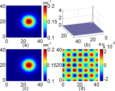

If we attempt to reconstruct an image that contains a sharp-edge target, more DCT coefficients have to be used. This is illustrated in Fig. 3a, where an image contains a square with sharp edges. The DCT coefficient map of this image is plotted in Fig. 3b. A reconstructed image using $6 \times 6$ DCT coefficients (one-seventh of total number of DCT coefficients) is presented in Fig. 3c. Figure 3d shows its corresponding relative error map. Notice that the error map of the reconstructed image reaches 20%, which is substantially larger than the one shown in Fig. 2d. In order to decrease the error down to 0.2%, we have to use $39 \times 39$ DCT coefficients. Figures 3e and 3f show the IDCT recovered image and the image errors, respectively.

Fig. 3

(a) A $42 \times 42 pixel$ absorption coefficient map with a square perturbation enclosed; (b) DCT coefficients of the absorption image (a); (c) an IDCT recovered image using $6 \times 6$ low-frequency DCT coefficients; (d) the relative error map of the recovered image (c); (e) an IDCT recovered image using $39 \times 39$ DCT coefficients; and (f) the relative error map of the recovered image (e).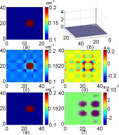

3.2.

OT with Parametric-DCT Method

To accurately calculate the photon propagation requires a finely discretized mesh. We found that in some cases, up to 10 discretized elements per photon mean free path are needed. Such a finely discretized mesh induces images that contain a very large number of pixels. The algorithm described in Sec. 2.2 treats each discretized element of an image as an independent variable. Therefore, the forward discretization results in a large number of unknowns for the inverse computation.

The image compression technique with DCT can help to reduce the number of these unknowns. We write the spatial distributed optical properties in a three-dimensional (3-D) domain as:

Eq. 9

μ_{a (s)} (x, y, z) ≃ \sum_{k_{x} = 0}^{K_{x}} \sum_{k_{y} = 0}^{K_{y}} \sum_{k_{z} = 0}^{K_{z}} A_{a (s)} (k_{x}, k_{y}, k_{z}) \cos (\frac{2 x + Δ x}{2 L_{x}} k_{x} π) \cos (\frac{2 y + Δ y}{2 L_{y}} k_{y} π) \cos (\frac{2 z + Δ z}{2 L_{z}} k_{z} π),

where

μ_{a (s)} (x, y, z)

is the absorption (or scattering) coefficients at

x = (x, y, z)

.

A_{a (s)} (k_{x}, k_{y}, k_{z})

represents DCT coefficients at spatial frequency

k_{x}

,

k_{y}

, and

k_{z}

in the

x

,

y

, and

z

directions.

L_{x}

,

L_{y}

, and

L_{z}

are the length in the

x

,

y

, and

z

directions.

K_{x}

,

K_{y}

, and

K_{z}

are the numbers of DCT coefficients to be used in reconstruction.

Δ x

,

Δ y

, and

Δ z

are the discretized resolutions.

With Eq. 9, the objective function that we want to minimize takes on the following form:

Eq. 10

\min Φ (A_{a}, A_{s}) = \frac{1}{2} \sum_{i = 1}^{N_{s}} \sum_{d = 1}^{N_{d}} {(P_{i, d} u_{i} - z_{i, d})}^{2},

where

A_{a}

and

A_{s}

are the DCT coefficients for

μ_{a}

and

μ_{s}

, respectively. Compared with Eq. 6, the reconstructed parameters changed from optical properties

(μ_{a}, μ_{s})

to DCT coefficients

(A_{a}, A_{s})

. Also, the regularization term is left out. Regularization terms, such as the Tikhonov regularization,¹⁶ tend to smooth images by removing high-spatial-frequency components. Using a parametric reconstruction technique based on the DCT expansion, the higher frequency components are automatically filtered out and hence the use of an extra regularization term is not needed.

To minimize the objective function in Eq. 10, we employ a quasi-Newton approach with BFGS updates of the Hessian matrix.¹⁷ The gradient of the objective function (10) can be written as:

Eq. 11

\frac{\partial Φ}{\partial A_{a (s)} (k_{x}, k_{y}, k_{z})} = \sum^{N} \frac{\partial Φ}{\partial μ_{a (s)} (x, y, z)} \cos (\frac{2 x + Δ x}{2 L_{x}} k_{x} π) \cos (\frac{2 y + Δ y}{2 L_{y}} k_{y} π) \cos (\frac{2 z + Δ z}{2 L_{z}} k_{z} π),

where

\partial Φ ∕ \partial μ_{a (s)} (x, y, z)

is the derivative of the objective function with respect to optical properties, and

N

is the number of total discretized elements. Details on how to obtain the derivative with respect to optical properties can be found in Ref. 8.

The overall flowchart for an image reconstruction algorithm that makes use of the parametric-DCT method is presented in Fig. 4 . By comparing this flow chart with the flow chart for the conventional MOBIIR approach shown in Fig. 1, one can easily see the main differences between these two methods. Both methods employ the same forward solver and use a quasi-Newton method to update their system parameters. However, in the DCT approach, the gradient of the objective function is calculate with respect to the DCT coefficients, while in the conventional MOBIIR scheme the gradient is calculated with respect to the optical properties. Subsequently, the updated DCT coefficients are used to update the optical properties using Eq. 9; and the new optical property values become input to the forward solver in the next iteration step.

Fig. 4

A flowchart of reconstructing a spatial distribution optical properties map with the parametric-DCT method.

3.3.

Number of DCT Coefficients

Choosing an appropriate number of DCT coefficients for the reconstruction is an important issue. The number of necessary DCT coefficients used to store and recover an image is determined by the smoothness of the image. The smoother an image is, the fewer DCT coefficients are required. As shown in Fig. 2 and Fig. 3, a sharp-edged object in an image requires more DCT coefficients. If we have some prior knowledge of the image features, we can choose a suitable number of DCT coefficients to represent the image and later use that number of DCT coefficients to perform the reconstruction. Such prior knowledge will help to improve the quality of the reconstructed images (see Sec. 4.3).

Some information about the number of DCT coefficients necessary for optical tomographic imaging can be gleaned from studies of resolution limits and minimal detectable object size in OT. These topics have been studied by several groups.^{3, 18, 19, 20, 21} These authors found that the achievable resolution depends on tissues’ size, geometry, optical properties, imaging modality and many other parameters. Pogue ²² argued that standard resolution testing is optimal when infinite contrast is used and hardware evaluation is the goal. However, deep tissue imaging of absorption or fluorescent contrast agents in vivo requires a more detailed analysis that takes tissue contrast into account. Overall, they found that for most biological tissues, a good approximation is to assume that the minimum detectable size is in the range of $1 ∕ 10$ of the outer diameter of the object imaged. For our analysis, this finding can be interpreted as to mean that smallest spatial variations in reconstructed optical tomographic images are in the range of $1 ∕ 10$ of the outer diameter.

Given this degree of spatial variation, we can estimate an approximate number of necessary DCT coefficients as follows. We define $K_{x}$ (or $y, z$ ) as the maximum number of DCT coefficients needed in one dimension, $Δ x$ (or $y, z$ ) as the resolution of an OT image along $x$ (or $y, z$ ) direction, and $L_{x}$ (or $y, z$ ) as the length of an OT image in $x$ (or $y, z$ ) direction. Then we can write:

Eq. 12

K_{x (or y, z)} = \frac{L_{x (or y, z)}}{λ ∕ 2} = \frac{L_{x (or y, z)}}{Δ x (or Δ y, Δ z)} .

Here, we define the wavelength

(λ ∕ 2)

of a cosine function as the limit of spatial variability

[Δ x (or Δ y, Δ z)]

. Assuming that

Δ x (or Δ y, Δ z)

is

1 ∕ 10 L_{x (or y, z)}

, as found by Pogue,²² we see that one needs approximately 10 coefficients for each dimensions. We used these considerations as a guide throughout our studies.

4. Numerical Examples

4.1.

Tissue Geometry

We illustrate the performance of the parametric-DCT reconstruction algorithm by using three-dimensional (3-D) numerical examples. The geometry of the problems considered in this work are shown in Fig. 5 . First, we consider a cylindrical computational domain defined as $D ≔ {{(x, y, z)}^{T} | {[{(x - 2.05)}^{2} + {(y - 2.05)}^{2}]}^{1 ∕ 2} ⩽ 2.05 cm; 0.0 ⩽ z ⩽ 3.0 cm}$ . Inside this domain, a cylindrical capsule (perturbation) is located defined by $D ≔ {{(x, y, z)}^{T} | {[{(x - 3.0)}^{2} + {(y - 3.0)}^{2}]}^{1 ∕ 2} ⩽ 0.7 cm; 1.2 ⩽ z ⩽ 2.2 cm}$ [see Fig. 5a]. The scattering coefficients and anisotropy factors of the background medium are identical to those of the cylindrical perturbation ( $μ_{s} = 40.0 {cm}^{- 1}$ , $g = 0.73$ ). The absorption coefficients of the background and cylindrical perturbation are $0.1 {cm}^{- 1}$ and $0.2 {cm}^{- 1}$ , respectively. The source modulation frequency is set to $ω = 300 MHz$ . Using the mesh generating software GID, the computational domain is discretized into 13,798 elements with 2723 nodes. The angular domain is discretized into 24 uniformly distributed directions with a full-level symmetry. This discretization yields a total number of 13,798 unknown parameters, if we consider to reconstruct the absorption optical properties on the discretized elements only. In this case, the measurement data are generated by a synthetic forward computation rather than real experiments. Two layers of sources and detectors are placed around the boundary, as illustrated in Fig. 5a. The two layers are separated by $1.0 cm$ . On each layer 12 sources (S12) and 12 detectors (D12) are evenly distributed. In totally, we will generate $S 24 \times D 24 = 576$ measurement data, which is far fewer than 13,798, the number of unknown discretized elements.

Fig. 5

A tissue-like phantom and source–detector geometries used in this study. The numerical phantoms shown in (a) and (b) mimic the experimental tissue geometry shown in (c). A cylinder with outer diameters of $4.1 cm$ contains a cylindrical perturbation of diameter $1.4 cm$ , which is located slightly off center. The perturbation is either a capsule of height $1.0 cm$ or a column with the same height as the outer cylinder. Optical properties and more details concerning this phantom are given in the text.

In a second set of studies, we consider another cylindrical domain, this time given by $D ≔ {{(x, y, z)}^{T} | {[{(x - 2.05)}^{2} + {(y - 2.05)}^{2}]}^{1 ∕ 2} ⩽ 2.05 cm; 0.0 ⩽ z ⩽ 5.0 cm}$ . The cylindrical perturbation is given by $D ≔ {{(x, y, z)}^{T} | {[{(x - 3.0)}^{2} + {(y - 3.0)}^{2}]}^{1 ∕ 2} ⩽ 0.7 cm; 0.0 ⩽ z ⩽ 5.0 cm}$ . Therefore, in this case both the height of the background cylinder and the perturbation are $5 cm$ [see Fig. 5b]. The perturbation has a uniform distribution along the $z$ direction. The discretization yields 23,221 unknown elements with 4512 nodes. We use 24 full-level symmetrical distribution directions as well. The examples chosen here only reconstruct images of absorption coefficients with fixed scattering coefficients. Scattering coefficients’ reconstruction can be implemented in a similar way.

4.2.

Image Evaluation Metrics

In the following, we will compare reconstruction results of the parametric-DCT approach to those obtained through the conventional MOBIIR algorithm. To quantify the reconstruction quality and the differences between the two approaches, we use the following imaging evaluation metrics:

1. Maximum error:
Eq. 13
$ε_{\max} = \max (ε_{1}, \dots, ε_{i}, \dots, ε_{N}) with ε_{i} = | μ_{i}^{r} - μ_{i}^{o} | .$
2. Normalized root mean square error:

Eq. 14

ε_{rms} = {[\frac{1}{N} \sum_{i = 1}^{N} (\frac{μ_{i}^{r} - μ_{i}^{o}}{μ_{i}^{o}})]}^{1 ∕ 2},

where

μ_{i}^{o}

and

μ_{i}^{r}

are the exact and reconstructed values on the discretized element

i

, respectively. We also employ these metrics to quantify the effects of the initial guesses and noise on reconstructed images.

4.3.

Image Reconstruction Results

4.3.1.

Reconstruction of a capsular perturbation

In this example, we varied the number of DCT coefficients to study their influence on the reconstruction results. To straddle the range of 10 coefficients as discussed in Sec. 3.3, we first fix the number of DCT coefficients in the $x y$ cross section $K_{x} \times K_{y} = 10 \times 10$ , and vary $K_{z} = 5$ , 10, 15. Next, we fix $K_{z} = 10$ and vary $K_{x} = K_{y} = 5$ , 10, 15. The initial absorption coefficients are set as $μ_{a} = 0.1 {cm}^{- 1}$ (background value).

Figure 6 shows the results obtained by varying the number of DCT coefficients in the $x y$ cross section. One can see that the reconstructed images with $K_{x} \times K_{y} \times K_{z} = 5 \times 5 \times 10$ [Figs. 6d, 6e, 6f] reproduce the shape of the perturbation; however, the background shows somewhat larger fluctuations when compared to the results obtained with $K_{x} \times K_{y} \times K_{z} = 10 \times 10 \times 10$ [Figs. 6g, 6h, 6i]. If we further increase $K_{x} \times K_{y}$ to $15 \times 15$ [Figs. 6j, 6k, 6l], the image quality deteriorates.

Fig. 6

3-D reconstruction results of the spatial distribution of $μ_{a}$ $({cm}^{- 1})$ using the parametric-DCT method with different numbers of DCT coefficients at $x y$ cross section. The images are extracted at the planes defined as (a), (d), (g), and (j): $z - 1.7 = 0.0$ ; (b), (e), (h), and (k): $y - 2.05 = 0.0$ ; (c), (f), (i), and (l): $x - 3.0 = 0.0$ . Here (a), (b), and (c) are cross-sectional images for the exact setup; (d), (e), and (f) for the parametric-DCT reconstructed images with DCT coefficient numbers $K_{x} \times K_{y} \times K_{z} = 5 \times 5 \times 10$ ; (g), (h), and (i) for the parametric-DCT reconstructed images with DCT coefficient numbers $K_{x} \times K_{y} \times K_{z} = 10 \times 10 \times 10$ ; (j), (k), and (l) for the parametric-DCT reconstructed images with DCT coefficient numbers $K_{x} \times K_{y} \times K_{z} = 15 \times 15 \times 10$ , respectively.

Figure 7 shows the reconstruction results obtained by fixing $K_{x} \times K_{y} = 10 \times 10$ and varying the number of DCT coefficients along the $z$ direction. When $K_{z} = 5$ , we observe [In Figs. 7d, 7e, 7f] that there are some fluctuation around the boundary. For $K_{z} = 15$ , the reconstructed images show more fluctuation in the background. Table 1 provides the related maximum error and the normalized mean square error. Overall, one can see that the combination of $K_{x} \times K_{y} \times K_{z} = 10 \times 10 \times 10$ gives the smallest errors. Therefore, we will use this number of coefficients $K_{x} \times K_{y} \times K_{z} = 10 \times 10 \times 10$ in the following simulations, where we study the influence of the initial guess and noise levels on the reconstruction results.

Fig. 7

3-D reconstruction results of the spatial distribution of $μ_{a}$ $({cm}^{- 1})$ using the parametric-DCT method with different numbers of DCT coefficients along the $z$ direction. The images are extracted at the planes defined as (a), (d), (g), and (j): $z - 1.7 = 0.0$ ; (b), (e), (h), and (k): $y - 2.05 = 0.0$ ; (c), (f), (i), and (l): $x - 3.0 = 0.0$ . Here (a), (b), and (c) are cross-sectional images for the exact setup; (d), (e), and (f) for the parametric-DCT reconstructed images with DCT coefficient numbers $K_{x} \times K_{y} \times K_{z} = 10 \times 10 \times 5$ ; (g), (h), and (i) for the parametric-DCT reconstructed images with DCT coefficient numbers $K_{x} \times K_{y} \times K_{z} = 10 \times 10 \times 10$ ; (j), (k), and (l) for the parametric-DCT reconstructed images with DCT coefficient numbers $K_{x} \times K_{y} \times K_{z} = 10 \times 10 \times 15$ , respectively.

Table 1

Errors of the reconstructed images using the parametric-DCT method with different numbers of DCT coefficients.

Kx×Ky×Kz	5×5×10	10×10×10	15×15×10	10×10×5	10×10×15
$ε_{\max}$	0.0499	0.0484	0.0632	0.0527	0.0498
$ε_{rms}$	0.0784	0.0744	0.0936	0.0749	0.0752

Next, we compare the results of the parametric-DCT reconstruction $(K_{x} \times K_{y} \times K_{z} = 10 \times 10 \times 10)$ with those of the conventional MOBIIR reconstruction (Figs. 8 and 9 ). Looking at Figs. 8d, 8e, 8f, we notice that using the conventional MOBIIR method the shape of the perturbation is distorted. Using the parametric-DCT method [see Figs. 8g, 8h, 8i], the shape of the perturbation is much smoother. The cross-line plots presented in Fig. 9 give the values of optical properties along the Cartesian coordinates crossing the center of the capsulized perturbation. This shows that the cross-line curves of the absorption values have a smooth bell shape when the parametric-DCT method is employed. Using the conventional MOBIIR method results in more fluctuating curves (Table 2 ).

Fig. 8

3-D reconstruction results of the spatial distribution of $μ_{a}$ $({cm}^{- 1})$ with the conventional MOBIIR method and the parametric-DCT method. The reconstructed cross-sectional images are extracted at the plane defined as (a), (d), and (g): $z - 1.7 = 0.0$ ; (b), (e), and (h): $y - 2.05 = 0.0$ ; (c), (f), and (i): $x - 3.0 = 0.0$ . Here, (a), (b), and (c) are cross-sectional images for the exact setup; (d), (e), and (f) for the conventional MOBIIR reconstruction; and (g), (h), and (i) for the parametric-DCT reconstruction, respectively.

Fig. 9

Cross-line plots of the reconstructed absorption coefficients of Fig. 8 at the line: (a) along the $x$ axis at the plane $z - 1.7 = 0.0$ ; (b) along the $y$ axis at the plane $z - 1.7 = 0.0$ ; (c) along the $z$ axis at the plane $x - 3.0 = 0.0$ .

Table 2

Errors of the reconstructed images using the parametric-DCT method and the conventional MOBIIR method.

	Capsule		Column
	Conventional	Parametric-DCT	Conventional	Parametric-DCT
	Conventional	Parametric-DCT	Conventional	(10×10×10)	(10×10×1)
$ε_{\max}$	0.0536	0.0484	0.0803	0.0563	0.0548
$ε_{rms}$	0.0770	0.0744	0.1581	0.1601	0.1435

4.3.2.

Reconstructions of a column perturbation

To compare experimental results with our numerical simulations, we consider a cylindrical medium with a cylindrical column perturbation [see Fig. 5b]. Given the results obtained in the previous section, we performed the reconstruction with with $K_{x} \times K_{y} \times K_{z} = 10 \times 10 \times 10$ . In addition, assuming that we know that there are no variation in the optical properties along the $z$ direction, we also performed reconstructions with $K_{x} \times K_{y} \times K_{z} = 10 \times 10 \times 1$ . Figure 10 shows the exact absorption maps [Figs. 10a, 10b, 10c], the reconstructed absorption maps using the parametric-DCT method [Figs. 10d, 10e, 10f, 10g, 10h, 10i], and the reconstructed absorption maps using the conventional method [Figs. 10j, 10k, 10l]. The cross-line plots of the optical properties of the reconstruction images are presented in Fig. 11 .

Fig. 10

3-D reconstruction results of the spatial distribution of $μ_{a}$ $({cm}^{- 1})$ with the conventional MOBIIR method and the parametric-DCT method for the column perturbation. The reconstructed cross-sectional images are extracted at the plane defined as (a), (d), (g), and (j): $z - 2.5 = 0.0$ ; (b), (e), (h), and (k): $y - 2.05 = 0.0$ ; (c), (f), (i), and (l): $x - 3.0 = 0.0$ . Here (a), (b), and (c) are cross-sectional images for the exact setup; (d), (e), and (f) for the parametric-DCT reconstruction with $K_{x} \times K_{y} \times K_{z} = 10 \times 10 \times 1$ ; (g), (h), and (i) for $K_{x} \times K_{y} \times K_{z} = 10 \times 10 \times 10$ ; and (j), (k), and (l) for the conventional MOBIIR reconstruction, respectively.

Fig. 11

Cross-line plots of the reconstructed absorption coefficients of Fig. 10 at the line: (a) along the $x$ axis at the plane $z - 2.5 = 0.0$ ; (b) along the $y$ axis at the plane $z - 2.5 = 0.0$ ; (c) along the $z$ axis at the plane $x - 3.0 = 0.0$ .

One can see that employing the prior information enhances the image quality [see Figs. 10d, 10e, 10f]. Fixing $K_{z} = 1$ leads to a uniform distribution of absorption coefficients along the $z$ direction. If we ignore this prior information and reconstruct with parameters $K_{x} \times K_{y} \times K_{z} = 10 \times 10 \times 10$ , we are still able to obtain smooth images. However, along the $z$ direction, the reconstructed perturbation has limited length and locates around the two source–detector planes. Information from above and below these two planes is limited. Last, we observe that the reconstructed images using the conventional MOBIIR method are much more noisy than the results obtained with the parametric image reconstruction method. The related values for the maximum errors and the root mean square errors are 0.0803 and 0.1581 for MOBIIR reconstruction and 0.0563 and 0.1601 for the parametric DCT method with $1010 \times 10$ coefficients (see Table 2).

4.4.

Effects of the Initial Guess on Reconstruction Results

At the heart of the inverse reconstruction for both the conventional MOBIIR and the parametric-DCT method is the quasi-Newton update, which is an optimization scheme for finding a local minimum. If the initial guess fed into the reconstruction algorithm is far away from the true minimum, it is difficult for the algorithm to converge to its real solution.¹⁷ To evaluate the sensitivity of the parametric-DCT reconstruction method to the choice of the initial guess, we performed numerical studies using the capsular perturbation. The number of DCT coefficients is fixed to $K_{x} \times K_{y} \times K_{z} = 10 \times 10 \times 10$ .

Figure 12 presents the reconstructed cross-sectional images with initial guesses varying from $μ_{a} = 0.10 {cm}^{- 1}$ (background value) to $μ_{a} = 0.05 {cm}^{- 1}$ . As expected, we observe that the stronger the initial guess deviates from the background value, the worse the images’ qualities are. However, even an initial guess 50% lower than the actual values still leads to a reasonable result. This cannot be said when the conventional MOBIIR scheme is applied. Figures 12j, 12k, 12l show a much more noisy reconstruction than Figs. 12g, 12h, 12i. Table 3 shows the errors and mean values of the reconstructed images. We define the images mean value as ${\bar{μ}}_{a} = \sum_{i}^{N} μ_{a} (i) ∕ N$ , with $N$ as the number of discretized elements. Comparing the parametric-DCT method with the conventional MOBIIR method at the initial guess $μ_{a} = 0.05 {cm}^{- 1}$ , one can find that the parametric-DCT method yields smaller errors and a closer mean value to the exact image. We define the mean value offset as $δ {\bar{μ}}_{a} = | {\bar{μ}}_{a}^{r} - {\bar{μ}}_{a}^{o} |$ , with ${\bar{μ}}_{a}^{r}$ and ${\bar{μ}}_{a}^{o}$ as the mean values of the reconstructed and exact images, respectively. We can see the reconstructed mean values with the parametric-DCT approach are less offset, as shown in the last row of Table 3. Overall, these results show that the parametric-DCT approach is much less sensitive to the choice of the initial guess than the conventional MOBIIR scheme.

Fig. 12

3-D reconstruction results of the spatial distribution of $μ_{a}$ $({cm}^{- 1})$ starting the iterations with different initial guesses. The cross-sectional images are extracted at the plane defined as (a), (d), (g), and (j): $z - 1.7 = 0.0$ ; (b), (e), (h), and (k): $y - 2.05 = 0.0$ ; (c), (f), (i), and (l): $x - 3.0 = 0.0$ . Here (a), (b), and (c) are the parametric-DCT reconstruction with initial guess $μ_{a}^{0} = 0.10 {cm}^{- 1}$ ; (d), (e), and (f) for the parametric-DCT reconstruction with initial guess $μ_{a}^{0} = 0.07 {cm}^{- 1}$ ; (g), (h), and (i) for the parametric-DCT reconstruction with initial guess $μ_{a}^{0} = 0.05 {cm}^{- 1}$ ; (j), (k), and (l) for the conventional MOBIIR reconstruction with initial guess $μ_{a}^{0} = 0.05 {cm}^{- 1}$ , respectively.

Table 3

Errors and mean values of reconstructed images with different initial guesses in the capsular perturbation case.

	Exact	Parametric-DCT			Conventional
$μ_{a}^{0}$	N/A	0.10	0.07	0.05	0.05
$ε_{\max}$	N/A	0.0484	0.0555	0.0625	0.0954
$ε_{rms}$	N/A	0.0744	0.1596	0.2457	0.2930
${\bar{μ}}_{a}$	0.1019	0.1023	0.0949	0.0903	0.0850
$δ {\bar{μ}}_{a}$	0	0.0004	$- 0.0070$	$- 0.0116$	$- 0.0169$

4.5.

Effects of Measurement Noise on Reconstruction Results

To study the effect of measurement noise on the parametric-DCT reconstructions, we purposely add a certain amount of random noise to the synthetically generated data. If $J_{i, d}$ is a synthetic measurement corresponding to the source $i$ and the detector $d$ , then the noisy data ${\bar{J}}_{i, d} = J_{i, d} (1 + δ_{i, d} N (0, 1) I_{[- 1, 1]})$ . Here, $N (0, 1)$ is a standard normal distribution, and $I [- 1, 1]$ is an interval indicator function that is equal to 1 in the interval of $[- 1, 1]$ and zero otherwise. The parameter $δ_{i, d}$ is the standard deviation of added noise, which we vary from 1% to 5%, which are typical values for OT measurement systems. We test the effect of this type of noise on the reconstruction results of a cylindrical domain with a capsulized perturbation (Fig. 5). Again, we chose the number of DCT coefficients as $K_{x} \times K_{y} \times K_{z} = 10 \times 10 \times 10$ .

The reconstruction results are shown in Fig. 13 . As expected, we see that as the standard deviation of the added noised increases, the quality of the reconstructed images decreases. When we add 5% noise, some artificial perturbations appear in the background area, while the reconstructed absorption values decrease in perturbation area. However, we also observe that the parametric-DCT reconstruction approach outperforms the conventional MOBIIR method at the same noise level [see Figs. 13g, 13h, 13i, 13j, 13k, 13l]. Using the conventional approach, we see artificial inhomogeneities in background area and the shape of reconstructed perturbation appears distorted. The maximum errors and normalized standard deviation errors with varying noise levels are presented in Table 4 . Overall, we find that the parametric-DCT method is less sensitive to noise.

Fig. 13

3-D reconstruction results of the spatial distribution of $μ_{a}$ $({cm}^{- 1})$ with different noise levels. The cross-sectional images are extracted at the plane defined as (a), (d), (g), and (j): $z - 1.7 = 0.0$ ; (b), (e), (h), and (k): $y - 2.05 = 0.0$ ; (c), (f), (i), and (l): $x - 3.0 = 0.0$ . Here (a), (b), and (c) are the parametric-DCT reconstruction without noise; (d), (e), and (f) for the parametric-DCT reconstruction with 2% noise; (g), (h), and (i) for the parametric-DCT reconstruction with 5% noise; (j), (k), and (l) for the conventional MOBIIR reconstruction with 5% noise, respectively.

Table 4

Errors of reconstructed images with different noise level in the capsule perturbation case.

	Parametric-DCT			Conventional
Noise level	No noise	2%	5%	5%
$ε_{\max}$	0.0484	0.0611	0.1103	0.3111
$ε_{rms}$	0.0744	0.1299	0.1596	0.2655

5. Image Reconstruction with Experimental Data

Last, we also tested our new parametric imaging reconstruction code with experimental data. The experimental data were acquired with a continuous wave dynamic near-infrared optical tomographic (DYNOT) system.²³ In this system, light from a laser diode (wavelength $λ = 760 nm$ is delivered to 24 source fiber bundles via an optical demultiplexing switch that allowed light to be sequentially delivered to different positions. The demultiplexor consists of a mirror mounted on a rotating stepper motor, which reflected light from the incoming laser source into different source fibers depending on the angular orientation of the mirror. Twenty-four detector fiber bundles were used to direct light to the detectors. Light was collected by silicon photodiodes, which were connected to a series of programmable amplifiers and a lock-in filter. Reported signal-to-noise ratio (SNR) is in the range of 0.5% to 5%, depending on the optical properties and tissue geometries. More details concerning this system can be found in Ref. 23.

The tissue-like phantom used in this study has a similar geometry compared to the preceding numerical setup with a column perturbation [see Sec. 4.3.2, Fig. 5c]. The background medium of this phantom consists of a 1% Intralipid solution. The cylindrical perturbation is made from a mix of 1% Intralipid and ink placed in a transparent straw. The scattering coefficients of the background and the perturbation are the same $μ_{s}^{b} = μ_{s}^{p} \sim 27.0 {cm}^{- 1}$ (Ref. 24). The absorption coefficients of the background and the perturbation are $μ_{a}^{b} \sim 0.023 {cm}^{- 1}$ and $μ_{a}^{p} > 0.1 {cm}^{- 1}$ , respectively.²⁵ The anisotropic factor $g \sim 0.73$ is close to water. The diameter of this perturbation $d \sim 0.6 cm$ is a little smaller than the size of numerical perturbation used in sections above.

The reconstructed absorption maps and corresponding cross-line plots are shown in Figs. 14 and 15 , respectively. For the parametric-DCT reconstruction, We used $K_{x} \times K_{y} \times K_{z} = 10 \times 10 \times 1$ DCT coefficients. We can see that the parametric-DCT approach outperforms the conventional MOBIIR method. Both the shape and absolute optical properties of the inhomogeneity are better recovered with the parametric-DCT method. This is in agreement with the findings of our numerical studies.

Fig. 14

3-D phantom experimental data reconstruction results of the spatial distribution of $μ_{a}$ $({cm}^{- 1})$ with the parametric-DCT method and the conventional MOBIIR method. The cross-sectional images are extracted at the plane defined as (a) and (d): $z - 2.5 = 0.0$ ; (b) and (e): $y - 2.05 = 0.0$ ; (c) and (f): $x - 3.1 = 0.0$ . Here (a), (b), and (c) are cross-sectional images for the conventional MOBIIR reconstruction; (d), (e), and (f) for the parametric-DCT reconstruction, respectively.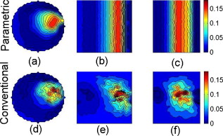

Fig. 15

Cross-line plots of reconstructed absorption coefficients of Fig. 14 at the line: (a) along the $x$ axis at the plane $z - 2.5 = 0.0$ ; (b) along the $y$ axis at the plane $z - 2.5 = 0.0$ ; (c) along the 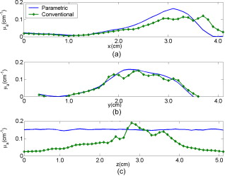$z$ axis at the plane $x - 3.1 = 0.0$ .

6. Discussion and Conclusions

We introduced a parametric image reconstruction approach to optical tomographic imaging, which makes use of the discrete-cosine transform (DCT) to represent the reconstructed images. This approach was implemented by adopting an existing model-based iterative image reconstruction (MOBIIR) scheme, which uses the frequency-domain equation of radiative transfer (ERT) as a forward model. We illustrated and analyzed the performance of the new code using synthetic as well as experimental data. We could demonstrate that the parametric-DCT reconstruction method allows us to substantially reduce the number of unknown image parameters and overall results in better quality of the reconstructed images, when compared to a conventional, nonparametric reconstruction techniques. In particular, the results show that DCT-based codes are less sensitive to noise in the data and to the choice of the initial guess needed in iterative image reconstruction schemes.

The number of unknowns in the imaging problem is reduced by expanding the reconstructed images into spatially varying 2-D or 3-D cosine functions of increasing order. If a typical image is discretized into pixels or voxels, the number of unknowns can be in the thousand and even millions, depending on the level of discretization. However, it has been shown by several groups that the detection limit of a heterogeneity is about $1 ∕ 10$ of the outer dimensions of the medium under consideration. This effectively means that variations of spatial properties in optical tomographic images are limited to about $1 ∕ 10$ of the outer dimensions. Our numerical results show that these variations can be captured with approximately 10 coefficients in each dimension, since the largest spatial frequency is proportional to one tenth of the base frequency. Therefore, using the parametric-DCT approach, only 10 unknowns (the expansion coefficients) per dimension need to be determined instead of the much larger number of pixels in an image.

If more and more expansion coefficients are used in the parametric-DCT algorithm, the images become increasingly similar to the images obtained with traditional nonparametric MOBIIR codes. In this case, the number of unknowns in parametric-DCT reconstruction approaches the number of unknowns in the MOBIIR method. Higher frequency components that seem to produce artifacts become visible. The reason for that is most likely that an overfitting takes places, and the many unknowns will “fit” the noise in the data. On the other hand, as we use fewer and fewer coefficients in the parametric code, the images become smoother, and high-frequency components disappear. Since fewer unknowns are used, images reconstructed with the parametric-DCT method appear in general smoother than images generated with MOBIIR codes that use a larger number of unknowns.

Another advantage of the parametric DCT approach is that these codes converge faster to the final result. For the examples considered in this paper, we observed up to 50% reduction in convergence times. The exact speed-up factor depends on the optical properties, problem geometry, and the ratio of the mesh size to the number of chosen DCT coefficients.

In this paper, we present results concerning the reconstruction of the spatial distribution of the absorption coefficients. However, the same approach can be applied to reconstruct the spatial distribution of scattering coefficients. As indicated in Eq. 9, the absorption coefficients and the scattering coefficients of an image can be expanded in the spatial-frequency domain individually. Thus, the number of DCT coefficients for the absorption coefficients and for the scattering coefficients become independent. The number of necessary DCT coefficients to obtain a good scattering coefficients map will depend on the expected spatial variations in a reconstructed image. It has been shown that the spatial variations in the scattering images are of the same order as the variations in the absorption images (see, e.g., Dehghani ²¹ and Pogue ²²). Therefore, one can expect that a similar number of DCT coefficients are needed for scattering images, and indeed we found the same general trends for scattering images as described in the paper for absorption images.

Last, although the examples presented in this paper were based on optical tomography using the frequency-domain ERT, the parametric-DCT method by nature is not limited to any particular light-propagation model. The parametric-DCT reconstruction techniques can also be applied to diffusion-theory-based optical tomography and other inverse problems, such as impedance tomography and microwave tomography.

Acknowledgments

This work was supported in part by the National Institute of Biomedical Imaging and Bioengineering (NIBIB—Grant No. R01 EB001900) and the National Institute of Arthritis and Musculoskeletal and Skin Diseases (NIAMS—Grant No. 2R01-AR046255), both of which are part of the National Institutes of Health (NIH).

References

1.

A. Corlu, T. Durduran, R. Choe, M. Schweiger, E. M. C. Hillman, S. R. Arridge, and A. G. Yodh, “Uniqueness and wavelength optimization in continuous-wave multispectral diffuse optical tomography,” Opt. Lett., 28 (23), 2339 –2341 (2003). https://doi.org/10.1364/OL.28.002339 0146-9592 Google Scholar

2.

G. Gulsen, B. Xiong, O. Birgul, and O. Nalcioglu, “Design and implementation of a multifrequency near-infrared diffuse optical tomography system,” J. Biomed. Opt., 11 (1), 014020 (2006). https://doi.org/10.1117/1.2161199 1083-3668 Google Scholar

3.

D. A. Boas, A. M. Dale, and M. A. Franceschini, “Diffuse optical imaging of brain activation: approaches to optimizing image sensitivity, resolution, and accuracy,” Neuroimage, 23 (S1), S275 –288 (2004). https://doi.org/10.1016/j.neuroimage.2004.07.011 1053-8119 Google Scholar

4.

M. M. Huang and Q. Zhu, “A dual-mesh optical tomography reconstruction method with depth correction usign a priori ultrasound information,” Appl. Opt., 43 (8), 1654 –1662 (2004). https://doi.org/10.1364/AO.43.001654 0003-6935 Google Scholar

5.

M. Schweiger and S. Arridge, “Image reconstruction in optical tomography using local basis functions,” J. Electron. Imaging, 12 (4), 583 –593 (2003). https://doi.org/10.1117/1.1586919 1017-9909 Google Scholar

6.

K. R. Rao and P. Yip, Discrete Cosine Transforms: Algorithms, Advantages, Applications, Academic Press, New York (1990). Google Scholar

7.

G. K. Wallace, “The jpeg still picture compression standard,” Commun. ACM, 34 (4), 30 –44 (1991). https://doi.org/10.1145/103085.103089 0001-0782 Google Scholar

8.

K. Ren, G. Bal, and A. H. Hielscher, “Frequency-domain optical tomography with the equation of radiative transfer,” SIAM J. Sci. Comput. (USA), 28 (4), 1463 –1489 (2006). https://doi.org/10.1137/040619193 1064-8275 Google Scholar

9.

L. Henyey and J. Greenstein, “Diffuse radiation in the galaxy,” Astrophys. J., 90 (16), 70 –83 (1941). https://doi.org/10.1086/144246 0004-637X Google Scholar

10.

E. E. Lewis and W. F. Miller, Computational Methods of Neutron Transport, 2nd ed.American Nuclear Society, La Grange Park, IL (1993). Google Scholar

11.

R. Eymard, T. Gallouet, and R. Herbin, “Finite volume methods,” Handbook of Numerical Analysis VII, 2nd ed.North-Holland, Amsterdam (2000). Google Scholar

12.

K. Ren, G. S. Abdoulaev, G. Bal, and A. H. Hielscher, “Algorithm for solving the equation of radiative transfer in the frequency domain,” Opt. Lett., 29 (6), 578 –580 (2004). https://doi.org/10.1364/OL.29.000578 0146-9592 Google Scholar

13.

A. E. Jacquin, “Image coding based on a fractal theory of iterated contractive image transformations,” IEEE Trans. Image Process., 1 (1), 18 –30 (1992). https://doi.org/10.1109/83.128028 1057-7149 Google Scholar

14.

A. Bratko, G. V. Cormack, B. Filipic, T. R. Lynam, and B. Zupan, “Spam filtering using statistical data compression models,” J. Mach. Learn. Res., 7 2673 –2698 (2006). 1532-4435 Google Scholar

15.

I. Daubechies, Ten Lecutres on Wavelets, SIAM, Philadelphia (1992). Google Scholar

16.

H. W. Engl, M. Hanke, and A. Neubauer, Regularization of Inverse Problems, Kluwer Academic Publishers, Dordrecht (1996). Google Scholar

17.

J. Nocedal and S. J. Wright, Numerical Optimization, Springer-Verlag, New York (1999). Google Scholar

18.

J. A. Moon, R. Mahon, M. D. Duncan, and J. Reintjes, “Resolution limits for imaging through turbid media with diffuse light,” Opt. Lett., 18 (19), 1591 –1593 (1993). https://doi.org/10.1364/OL.18.001591 0146-9592 Google Scholar

19.

D. J. Hall, J. C. Hebden, and D. T. Delpy, “Evaluation of spatial resolution as a function of thickness for time-resolved optical imaging of highly scattering media,” Med. Phys., 24 (3), 361 –368 (1997). https://doi.org/10.1118/1.597904 0094-2405 Google Scholar

20.

D. A. Boas, M. A. O’Leary, B. Chance, and A. G. Yodh, “Detection and characterization of optical inhomogeneities with diffuse photon density waves: a signal-to-noise analysis,” Appl. Opt., 36 (1), 75 –92 (1997). https://doi.org/10.1364/AO.36.000075 0003-6935 Google Scholar

21.

H. Dehghani, B. W. Pogue, S. Jiang, B. Brooksby, and K. D. Paulsen, “Three-dimensional optical tomography: resolution in small-object imaging,” Appl. Opt., 42 (16), 3117 –3128 (2003). https://doi.org/10.1364/AO.42.003117 0003-6935 Google Scholar

22.

B. W. Pogue, S. C. Davis, X. Song, B. A. Brooksby, H. Dehghani, and K. D. Paulsen, “Image analysis methods for diffuse optical tomography,” J. Biomed. Opt., 11 (3), 033001 (2005). https://doi.org/10.1117/1.2209908 1083-3668 Google Scholar

23.

C. Schmitz, M. Locker, J. Lasker, and A. Hielscher, “Instrumentation for fast functional optical tomography,” Rev. Sci. Instrum., 73 (2), 429 –439 (2002). https://doi.org/10.1063/1.1427768 0034-6748 Google Scholar

24.

I. Driver, J. W. Feather, P. R. King, and J. B. Dawson, “The optical properties of aqueous suspensions of intralipid, a fat emulsion,” Phys. Med. Biol., 34 1927 –1930 (1989). https://doi.org/10.1088/0031-9155/34/12/015 0031-9155 Google Scholar

25.

S. J. Madsen, M. S. Patterson, and B. C. Wilson, “The use of india ink as an optical absorber in tissue-simulating phantoms,” Phys. Med. Biol., 37 985 –993 (1992). https://doi.org/10.1088/0031-9155/37/4/012 0031-9155 Google Scholar

Citation Download Citation

Xuejun Gu, Kui Ren, James M. Masciotti, and Andreas H. Hielscher "Parametric image reconstruction using the discrete cosine transform for optical tomography," Journal of Biomedical Optics 14(6), 064003 (1 November 2009). https://doi.org/10.1117/1.3259360

Published: 1 November 2009

Access the abstract

JOURNAL ARTICLE
11 PAGES

DOWNLOAD PAPER SAVE TO MY LIBRARY

GET CITATION

CITATIONS

Cited by 13 scholarly publications.

Explore citations on Lens.org

RIGHTS & PERMISSIONS

Get copyright permission Get copyright permission on Copyright Marketplace

KEYWORDS

Image restoration

Absorption

Optical properties

Optical tomography

Image compression

Reconstruction algorithms

Scattering

1.

Introduction

2.

Frequency Domain Optical Tomography with the ERT

2.1.

The Forward Problem

1.

Eq. 2

Eq. 3

Eq. 4

Eq. 5

2.2.

The Inverse Problem and Conventional MOBIIR Methods

Eq. 6

Fig. 1

3.

Parametric Reconstruction with the DCT

3.1.

Image Compression with DCT

7.

8.

Fig. 2

Fig. 3

3.2.

OT with Parametric-DCT Method

Eq. 9

Eq. 10

Eq. 11

Fig. 4

3.3.

Number of DCT Coefficients

Eq. 12

4.

Numerical Examples

4.1.

Tissue Geometry

Fig. 5

4.2.

Image Evaluation Metrics

Eq. 13

Eq. 14

4.3.

Image Reconstruction Results

4.3.1.

Reconstruction of a capsular perturbation

Fig. 6

Fig. 7

Table 1

Fig. 8

Fig. 9

Table 2

4.3.2.

Reconstructions of a column perturbation

Fig. 10

Fig. 11

4.4.

Effects of the Initial Guess on Reconstruction Results

Fig. 12

Table 3

4.5.

Effects of Measurement Noise on Reconstruction Results

Fig. 13

Table 4

5.

Image Reconstruction with Experimental Data

Fig. 14

Fig. 15

6.

Discussion and Conclusions

Acknowledgments

References

Show All Keywords

Keywords/Phrases

Search In:

Publication Years