1.

Introduction

Optical coherence tomography (OCT) is an imaging modality that uses reflected near-infrared light to obtain micron-scale, depth-resolved images of tissue. It can be used to capture a cross sectional or 3-D volume image. When properly calibrated, OCT can be used for quantitative measurements. Because OCT is nondestructive and highly sensitive, it is ideal for in-situ measurements of low contrast and/or highly scattering objects. Because OCT instruments can be rapid-scanning, small, robust, and relatively low cost, they are adaptable to the laboratory, clinical, or industrial environment.

OCT has been used for a variety of biomedical metrology applications including measuring the thickness of cartilage around joints,¹ the thickness of the retinal nerve fiber layer,² and thickness of the cornea.^{3, 4, 5, 6} OCT has also been used to evaluate the results of corneal refractive therapy, in which the patient wears rigid contact lenses overnight to reshape the cornea.⁷ Dynamic information can also be obtained, such as evaluating contact lens movement caused by blinking.⁸

OCT can also be used as a quality control tool to evaluate biological and nonbiological materials. For example, the cellular integrity of a tissue-engineered vascular graft could be ascertained prior to implantation.⁹ While OCT is ideally suited to imaging biological tissues, it is also appropriate for other translucent materials. Examples include imaging the fiber architecture of glass-reinforced polymer composites,¹⁰ analyzing dentures,¹¹ and imaging ceramic glazes.¹² Negrutiu ¹¹ used OCT to noninvasively examine dentures made with different molding techniques for defects. OCT was used by Yang ¹² to acquire images of the glaze subsurface that can provide insight into the technology used to manufacture the ceramic piece. In all of these applications, OCT was able to nondestructively assess the quality of a sample by providing images of subsurface structures.

We are interested in the development of OCT as a metrology tool for development and quality control of contact lenses. Deviation from design parameters and manufacturing variance could potentially be determined with OCT. There are several unique difficulties to overcome when measuring contact lenses. A majority of the contact lens market is in soft lenses, and soft lenses deform when exposed to air long enough to dry out. Therefore, the lenses must be imaged while submerged in a bacteria-resistant saline solution so that they retain their shape. Once submerged, the contact lens is difficult to keep stationary for consecutive measurements. The saline submersion also makes imaging difficult because the refractive indices of contact lenses and saline solution are similar. The current standard technique for measuring the thickness of a contact lens at a single arbitrary point is to use a low-force dial gauge.¹³ The final thickness measurement requires five repeated dial gauge measurements in air with the contact lens returned to saline solution in between each measurement. The drawback to this method is the length of time required for a single thickness measurement. Another widely used thickness measurement technique involves physically taking a cross sectional slice of the contact lens and placing the slice under a microscope for manual measurement. This technique has several drawbacks. First, the number of cross sectional slices that can be taken from a single lens is limited, which limits the number of measurements possible. Second, the method is destructive, so a contact lens must be sacrificed to perform the measurement. Third, the method is slow and requires a skilled technician to perform the measurements manually.

One specific quality control issue is a consequence of mechanical variations in the contact lens manufacturing process called prism. The prism referred to here is mechanical prism, which is not the same as optical prism. For this application, prism is defined as the difference between the largest and smallest thickness measurements, taken at a given distance from the contact lens edge, over a complete $360\mathrm{deg}$ rotation. Toric contact lenses are designed intentionally with a nonrotationally symmetric shape for patients with astigmatism. Prism can be used intentionally as a ballast to keep toric contact lenses from rotating while on the eye.¹⁴ Prism caused by mechanical variations, however, is unintentional and must be characterized to minimize it. On a spherical lens, the prism by design should be zero. In reality, however, the prism of a spherical lens is random, as is the angle of maximum thickness differential.

As a coherent imaging technique, OCT images suffer from speckle and may be low contrast and/or noisy. Therefore, care must be taken in the development of automated measurement algorithms. The semiautomatic algorithm for locating cartilage boundaries described in Ref. 1 used the rotational kernel transformation (RKT) technique for removing noise from the image, followed by Sobel edge detection and user-aided edge linking. Attempts to measure retinal nerve fiber layer thickness using OCT have produced many different segmentation techniques specialized for OCT images. Blumenthal ² measured retinal nerve fiber thickness using a commercially available OCT system that automatically segmented the OCT image using a thresholding technique. The boundaries of the retinal nerve fiber layer were found by smoothing each axial scan and locating the first points in the scan above a chosen threshold. Another example of automatic retinal nerve fiber location is Ref. 15. Bagci, Ansari, and Shahidi used an algorithm that first aligned the A-scans based on feature points found using a modified version of the Canny algorithm. Next, they applied a directional smoothing filter to the aligned image to smooth in the lateral direction while preserving edge transitions in the axial direction. Edge detection was then applied to the resulting smoothed image to locate six layers within the retina. Yet another approach to finding retinal nerve fiber layer boundaries is the use of a Markov boundary model.¹⁶ Koozekanani, Boyer, and Roberts used a 1-D second derivative of Gaussian to locate initial boundary locations for each A-scan. The Markov boundary model is used to improve the initial boundary locations by making physical assumptions about the relative location of adjacent boundary pixels. These approaches are appropriate for their applications, but images of contact lenses have unique properties different from cartilage or retina, so a new automated image analysis method needed to be developed.

The ability to nondestructively measure the prism of contact lenses can lead to more information about the manufacturing process, which in turn may lead to improvements to the final product. OCT appears to be well suited for this task. An algorithm has been developed that automatically analyzes a dataset containing OCT cross sectional images taken $360\mathrm{deg}$ around the contact lens. A custom contact lens imaging fixture was built, and a commercially available OCT system was used to develop and test the algorithm.

2.

Materials and Methods

2.1.

Optical Coherence Tomography Setup

A commercially available spectral domain OCT system (Thorlabs OCT930SR, Thorlabs, Newton, New Jersey) was used throughout this study. The system used a light source with a center wavelength of $930\mathrm{nm}$ and a bandwidth of $100\mathrm{nm}$ . The axial and transverse optical resolutions were 6.2 and $9.2\mu \mathrm{m}$ , respectively. Image depth was fixed at $1.6\text{-}\mathrm{mm}$ optical depth with $512\text{pixels}$ . The image width and number of pixels was adjustable but set to a width of $2\mathrm{mm}$ and $1000\text{pixels}$ for the duration of the study. Therefore, the pixel size was smaller than the optical resolution. This system acquired cross sectional images only, so external movement of the sample or the imaging probe was required to obtain volumetric data.

A stable fixture was designed to position the contact lens and enable rotation of the probe to take multiple images of the contact lenses. The cuvette was fitted with a v-shaped rubber wedge to hold the contact lens in place. Since deformation can occur if the contact lens is resting on its apex, the contact lens rested on its circumference with the apex pointing up.

Measuring prism requires measuring the thickness all the way around the contact lens at a fixed distance from the edge. The distance used for this experiment was $0.3\mathrm{mm}$ from the lens edge. Since the contact lens rested on its edges in the cuvette, the imaging probe was placed underneath the cuvette, pointing upward. The optical axis was placed at an angle of about $20\mathrm{deg}$ from the surface normal of the cuvette glass, as shown in Fig. 1 . The angle was used both to minimize reflection from the cuvette glass and to maximize the signal from the contact lens surfaces.

Fig. 1

Diagram of imaging fixture. The imaging probe was mounted to a rotation stage at an angle of $20\mathrm{deg}$ from vertical. The center of rotation of the rotation stage was aligned to match the center of the contact lens.

The rubber wedge in the cuvette prevented lateral motion, but not rotational motion. Therefore, the cuvette was held stationary while the probe rotated $360\mathrm{deg}$ to acquire all of the images in a set. An automated motorized rotation stage was used for maximum accuracy and repeatability. As shown in Fig. 2 , the contact lens was always oriented in the same way relative to the cuvette. This provided a consistent reference point for the rotation angle.

Fig. 2

There are markings on the contact lens at the angles shown, along with some text identifying the contact lens. These markings are used to obtain a consistent orientation inside the cuvette.

3.

Image Analysis

A Matlab program (Matlab, Natick, Massachusetts) was written to automatically analyze a single OCT image and measure the thickness of a contact lens $0.3\mathrm{mm}$ from the edge. The four main steps performed to make a thickness measurement include: 1. defining the contact lens, cuvette glass, and saline regions; 2. correcting refraction; 3. finding the measurement point and calculating the thickness; and 4. determining if the measurement was valid.

3.1.

Segmentation

The first major step of the algorithm was to accurately break the image into regions corresponding to the contact lens, the cuvette glass, and the saline solution, as defined in Fig. 3 . The regions can be clearly defined by boundary lines corresponding to the glass-saline interface and the contact lens-saline interfaces. Therefore, defining these lines was sufficient to completely segment the image into the required regions. Prior to searching for the cuvette glass boundary, the program performed three image preparation tasks.

Fig. 3

Region of interest for the final segmentation results are: cuvette glass, saline solution, and contact lens.

3.1.1.

Presegmentation image processing

First, the image was scaled for square pixels so that the error would not be magnified in one dimension over the other. The settings used to acquire the images in this work produced pixels that are $3.1\mu \mathrm{m}$ tall by $1.8\mu \mathrm{m}$ wide, as determined by taking images of a calibration target. The image was up-sampled using bilinear interpolation, so that each pixel measured $2.0\times 2.0\mu \mathrm{m}$ .

Second, the image was automatically cropped around the contact lens. Cropping was necessary for removing unwanted complications such as the rubber wedge or image artifacts. Cropping also reduced computation time, because all subsequent calculations had fewer pixels to process. The cropping algorithm located the approximate location of the contact lens in the image by estimating the derivative of a smoothed plot of the average intensity of each image column. The left-most local maximum of a sufficiently smoothed brightness plot corresponded with the location of the contact lens. Then everything outside of a $1000\text{-pixel}$ -wide window centered on the contact lens was removed. The resulting cropped image needed to be wide enough to safely encompass the contact lens and tall enough so that the $0.3\text{-}\mathrm{mm}$ measurement point was guaranteed to be in view.

The third and final image preparation task was the application of a median filter with a $5\times 5$ kernel. This removed most of the salt and pepper noise from the image, providing a much cleaner result for the following steps.

3.1.2.

Cuvette glass location

Next, the algorithm found the edge of the cuvette glass, which was assumed to be a straight line. The search required the following steps: 1. thresholding, 2. morphology, and 3. Hough transform. A threshold was used to create a bilevel image from the grayscale image. The threshold was determined using Otsu’s method.¹⁷ The resulting bilevel image was processed using binary closing with a $1\times 15\text{pixel}$ structuring element to make sure the glass line was continuous, which resulted in the image shown in Fig. 4 . This image was then skeletonized, which reduced all of the shapes down to one pixel wide. Then the Hough transform was used to locate the cuvette glass edge.¹⁸ The skeletonization ensured that the line found by the Hough transform was in the center of the cuvette glass boundary. The final result for the cuvette glass search is shown in Fig. 4, where the line representing the cuvette glass edge is shown in black.

Fig. 4

(a) Processed bilevel image. (b) The cuvette glass surface search result is shown, with the black line indicating the location and angle of the modeled surface, as computed by the segmentation algorithm.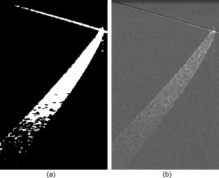

Before searching for the contact lens inner and outer edges, the image was rotated and shifted so that the cuvette glass was horizontal and located directly at the top of the view. The rotated image was then cropped further to a height of $800\text{pixels}$ , where the signal from the contact lens is too low to be visible. The rotation simplified the refraction correction calculations and improved the visual qualities of the final result.

3.1.3.

Contact lens boundary locations

Next, the four steps performed by the algorithm to locate the inner and outer edges of the contact lens were: 1. applying the threshold to create a mask, 2. processing the mask using binary morphology, 3. searching along the edges of the mask for edge points, and 4. fitting a polynomial to the inner edge and applying smoothing to the outer edge data points. A novel method for locating the edges of the contact lens was chosen rather than traditional edge detection such as Sobel or Canny. The reason for this choice was the speckle pattern of the contact lens in the OCT image. The contact lens did not appear as a solid structure; it showed up instead as a collection of large speckles with visible gaps between them, which can be seen in Fig. 3. It was assumed that the true contact lens edge existed along the centers of the outermost speckles. Based on this assumption, standard edge detection or threshold approaches could not locate the true contact lens edge as accurately as the algorithm we used.

The threshold step for identifying the contact lens edges was not as straightforward as the thresholding described previously for locating the cuvette glass. Locating and applying a threshold using the gray-level image was too sensitive to variations in signal-to-noise ratio (SNR) between images and other image artifacts. Instead, prior to finding a threshold, a texture analysis approach was used to improve the robustness of the search. This approach worked well, because the texture of the contact lens was clearly different from the texture of the saline solution, and that difference was independent of any variations in brightness, contrast, or SNR. One standard method of characterizing texture in an image is entropy.¹⁸ At every pixel in the rotated, cropped, gray-level image, the local entropy was calculated using a disk-shaped structuring element with a radius of five pixels. Each pixel in the image was replaced with its local entropy value, creating an entropy map. Again, using Otsu’s method, an ideal threshold was found and applied to the entropy map to create a bilevel image, which was used as a mask [see Fig. 5 ]. The resulting mask was refined using binary morphology operations, resulting in the final mask shown in Fig. 5.

Fig. 5

(a) Mask after threshold is applied to an entropy mask. (b) Mask in (a) processed using binary morphology to remove unwanted artifacts and leave only the contact lens visible.

Once the mask was complete, the algorithm began searching for data points along the inner and outer edges of the contact lens. The mask was applied to the cropped, rotated, gray-level image using element-by-element multiplication. As stated previously, it was assumed that the true edge of the contact lens existed in the center of the outermost speckles in the contact lens region. The algorithm searched along the inner and outer edges of the mask for the brightest pixel in a $7\times 7\text{pixel}$ region. The $7\times 7\text{pixel}$ area corresponded roughly with the size of the speckles, where it was assumed the brightest pixel corresponded with the centroid of the speckle.

After the inner and outer edge data points were collected, the algorithm fitted a third order polynomial to the inner surface using least squares regression. A polynomial was used for the inner surface so that the refraction correction algorithm described next could accurately calculate the surface normals. The outer edge points were smoothed instead of having a polynomial fit to them, because there was no need for a closed form representation of the outer surface. Also, the outer surface was often shaped in a way that would not allow for a simple functional representation of the surface. Robust Loess smoothing was used to smooth the outer surface data points, using a span of 30% of the data points as described in Ref. 19. The resulting segmentation result is shown in Fig. 6 , where the contact lens edges are shown in black.

Fig. 6

Final segmentation result with black lines indicating modeled inner and outer contact lens surfaces as computed by the segmentation algorithm.

3.2.

Refraction Correction

For consistency, the “inner” contact lens surface refers to the surface that sits against the eye, while the “outer” contact lens surface refers to the surface that is exposed to the air. The three regions in the image—contact lens, saline, and cuvette—each had a different refractive index. There were three surfaces that refracted light: the interface between air and the angled cuvette glass, the interface between the cuvette glass and the saline solution, and the inner contact lens surface. The outer contact lens surface refracted light as well, but there was nothing of interest beyond the outer surface, so no correction was necessary. The purpose of the algorithm was to locate precisely where the contact lens surfaces were and describe their shape in physical space. Since the cuvette glass was removed from the image during the location and image rotation step, the only surfaces that had to be corrected were the inner and outer contact lens surfaces. The refraction caused by the cuvette glass was taken into account during the calculation to determine the angle of the incoming rays from the top of the image. Westphal performed refraction correction on entire OCT images using a method based on Fermat’s principle of least time.²⁰ They used Fermat’s principle because their images had multiple curved surfaces, and the path of the beam through the sample could not be determined a priori.

In our application, the only refracting curved surface of interest was the inner contact lens surface, so the path of the beam could be computed for each surface using a ray-tracing model and Snell’s law. Also, there was no need in this application to correct the entire image. First, the inner contact lens surface was corrected followed by the outer contact lens surface. For each point along the surface of interest, the incoming ray was modeled as a group of line segments. The number of line segments corresponded to the number of refracting surfaces the light traveled through. Another line segment must be added to the model to account for the change in angle and the change in path length caused by each interface between materials with different refractive indices. Thus, the model for the incoming rays for the inner surface contained one line segment, and the model for the incoming rays for the outer surface contained two line segments. Each line segment was corrected for angle and length. The angle was computed using Snell’s law, and the length was computed by dividing the length of the line segment by the index of refraction of the material.

Once complete, the refraction correction algorithm produced a set of discrete data points for the inner and outer surfaces of the contact lens. The set of data points corresponding to the inner surface was modeled by a polynomial using least squares regression, and the outer surface data points were smoothed using robust Loess smoothing. The refraction corrected surfaces are shown in Fig. 7 as the solid white lines closest to the top of the image.

Fig. 7

Final measurement result, with white solid lines indicating refraction corrected contact lens surface models, and dashed white line indicating where the thickness measurement was taken.

4.

Results

4.2.

Accuracy

The nondestructive OCT thickness measurement technique presented here is meant to replace a destructive thickness measurement technique that requires the contact lens to be sliced. A thin slice of the contact lens was made by placing two blades close together and cutting across the center of the contact lens. This process could only be reliably performed once more after the first slice, producing a total of four measurement data points at the $0.3\text{-}\mathrm{mm}$ position. The slices were placed under a microscope and the thickness was measured manually. We compared this process to the OCT technique by taking OCT images of six contact lenses and then performing the manual microscope measuring technique. The angles for the measurements were matched using the markings on the contact lens shown in Fig. 2. Each lens was imaged three times at increments of $10\mathrm{deg}$ . This produced 108 images per lens. Once the OCT images were taken, the lenses were sliced and measured under a microscope. The slicing technique only produced four measurements per lens, so there are only four angles on each lens to compare the two methods. A histogram is given in Fig. 8 that shows the distribution of the difference between the two methods. A negative difference indicates that the OCT measurement was smaller than the microscope measurement. The mean difference is $-1.3\mu \mathrm{m}$ . The standard deviation of the difference is $1.7\mu \mathrm{m}$ , and the range between the maximum and minimum difference is $9.0\mu \mathrm{m}$ . Note that the three data points in the $-6\text{-}\mu \mathrm{m}$ bin all correspond to the same microscope measurement, because three OCT measurements were taken at each angle. Out of 648 images, 53 of them segmented incorrectly. Images taken at 45 and $135\mathrm{deg}$ were not expected to segment correctly because the contact lens was touching the rubber wedge inside the cuvette in these images, preventing any possibility of an accurate segmentation. Of the 53 segmentation errors, 24 were located adjacent to $(\pm 5\mathrm{deg})$ the 45- and $135\text{-}\mathrm{deg}$ points, 25 had data acquisition problems, and four were segmentation errors caused by the algorithm.

Fig. 8

Histogram of the difference between the OCT measurement and the microscope measurement. The bin values represent the difference between automated OCT measurements and manual microscope measurements of a specific lens at a specific angle. Computed using [OCT measurement]–[microscope measurement]=difference.

Figure 9 shows one example of a full thickness profile, including the microscope section results. The thickness profile has not been smoothed. The gaps in the profile occurred at angles of 45 and $135\mathrm{deg}$ , where the contact lens was touching the rubber wedge inside the cuvette and the algorithm could not determine where the contact lens ended and the rubber wedge began. The data points are located at the average of the three thickness values, and the error bars show the minimum and maximum measurements at each angle.

Fig. 9

Thickness profile data for a single contact lens.

5.

Discussion

The thickness measurement algorithm was able to accurately measure the thickness of a contact lens at $0.3\mathrm{mm}$ from the edge. The algorithm was able to process, crop, segment, correct refraction, and measure thickness without the need for user input.

The image preprocessing steps were simple to implement and left as much of the raw image data intact as possible. The image was up-sampled to achieve square pixels without any loss of data using bilinear interpolation, which was the best compromise between accuracy and speed.

One issue that can contribute error to quantitative OCT measurements is nontelecentric scanning. If the optics of the OCT system are not telecentric, then a sample with a straight edge will appear curved in the resulting OCT image. The refraction correction algorithm described by Westphal corrects for nontelecentric scanning in addition to refraction.²⁰ Our software does not make any telecentricity corrections to the image, because the Thorlabs OCT system is designed to be telecentric up to a maximum software limited image width of $10\mathrm{mm}$ . Our images were only $2\mathrm{mm}$ wide, and at this width the Thorlabs OCT system shows no detectable curvature caused by lack of telecentricity. Therefore, the assumption that the cuvette glass edge is a straight line in the image is valid, as shown in Fig. 4.

Accurately locating the contact lens surfaces was a key requirement for measuring thickness. The texture-based thresholding technique used for segmentation proved to be a reliable way of initially locating the contact lens in the image. None of the errors were caused by an incorrect or inadequate initial segmentation. Based on the assumptions that the contact lens surfaces are smooth and lie along the centers of the outermost speckles, the algorithm estimated the location of the contact lens surfaces with subpixel precision. Visual inspection revealed that the lines drawn by the software to mark the locations of the contact lens surfaces were in fact located directly on the centers of the outer speckles.

The refraction correction algorithm was verified indirectly by comparing the results of the OCT thickness measurement with the microscope thickness measurement. The similarity between the microscope results and the OCT results suggests that the refraction correction was performing correctly. No extra calibration factors were used to adjust the refraction correction calculations. Instead, calibration was performed by scaling the original acquired image in the horizontal and vertical directions by an amount determined by taking images of a calibration target. Also, the refractive indices of the materials visible in the OCT image were all measured separately, without using OCT. The fact that the largest difference between the OCT and microscope measurements was about the same as the optical resolution of the OCT system suggests that the refraction correction method is accurate to at least the resolution of the OCT system.

Since prism is a differential measurement between the extremes of the thickness profile, we could not afford to include bad data points in the dataset. Instead of removing data points based on whether the thickness measurement was inside expected boundaries, bad data points were identified based on the segmentation results. The shape of contact lenses dictates that the inner and outer surfaces will have almost the same slope at any particular point through the lens. Therefore, if the slopes of the inner and outer surfaces are not within 35% of each other at the measurement point, then the thickness is not included in the final dataset. Any gaps that this leaves in the thickness profile can be filled in by interpolating the thickness profile data.

A known issue with our setup is the inability to measure the contact lens thickness at angles within about $5\mathrm{deg}$ of 45 and $135\mathrm{deg}$ , where the contact lens touches the rubber wedge. If the maximum or minimum thickness lay at one of these angles, then the accuracy of the prism measurement depends on the extrapolation method for filling in these portions of the thickness profile. Another drawback to this technique is the requirement that the contact lens be placed in a glass cuvette filled with saline solution. While this technique is nondestructive, the lens must still be taken out of its mold or packaging to be measured.

Future applications for OCT as a contact lens metrology device include further development toward implementing OCT in the manufacturing line. The first step has already been completed by automating both image acquisition and image analysis. However, as mentioned before, the current technique requires the contact lens to be placed into a glass cuvette prior to measurement. In the future, it would be desirable for the OCT measurements to be made on a lens in the mold or in its final packaging.

6.

Conclusion

The results show that OCT can be used to accurately measure the thickness of contact lenses. The benefits of using OCT and our automated algorithm include nondestructive imaging, high sensitivity, speed, and no need for user input. The thickness measurement algorithm is able to accurately measure the thickness of a contact lens $0.3\mathrm{mm}$ from the edge. The algorithm is able to process, crop, segment, correct refraction, and measure thickness without the need for user input. The entire process takes $6\min$ and $55\sec$ to produce a report for 36 measurements. The acquisition alone takes $1\min$ $35\sec$ , so the majority of the time is spent on image analysis. The algorithm is implemented in Matlab. The analysis time could be decreased by translating the code to a compiled programming language such as C.

The OCT thickness measurements are very close to manually sectioned microscope thickness measurements. The OCT technique is nondestructive and allows for a much finer angular resolution for the resulting thickness profile. Assuming an accurate thickness measurement, a finer angular resolution will provide a more accurate prism measurement. Unlike the manual sectioning technique and other contact lens thickness measurement techniques, it may be possible to employ OCT instruments in the manufacturing line to automatically determine prism without sacrificing any contact lens samples. Two possible approaches could be used for imaging contact lenses on the manufacturing line. One approach is to image the contact lenses inside the mold. This approach would require greater imaging depth and more complicated image processing algorithms than we used. Another approach would involve imaging the contact lenses while they are submerged in saline solution, after they are removed from the mold. This approach would require the fastest possible imaging speed and less reliance on perfect alignment of the contact lens with the imaging probe. Other scanning topologies and packaging materials could be investigated to achieve the highest possible accuracy and shortest possible measurement time.