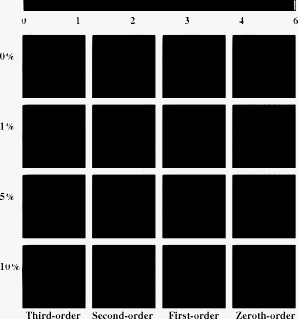
1.

Introduction

Optoacoustic imaging is a hybrid imaging technique that has attracted a lot of attention in recent years. It is based on the thermoacoustic effect, which refers to acoustic wave generation on absorption of pulsed optical energy by a medium. A slight rise in temperature of the medium due to the absorption of the incident electromagnetic wave results in thermoelastic expansion. This thermoelastic expansion and then contraction due to the pulsed electromagnetic waves leads to the generation of acoustic waves. Under the constraints of thermal and stress confinement, this thermal expansion leads to a rise in pressure, $p(\mathbf{r},t)$ , that satisfies the three-dimensional inhomogeneous wave equation¹

However, the speed of sound in tissues can vary from $1350\mathrm{m}∕\mathrm{s}$ (in fat) to about $1700\mathrm{m}∕\mathrm{s}$ (for skin) for ultrasound waves in the $1–10\mathrm{MHz}$ range.² Using a constant speed of sound in image reconstruction can result in image distortion and poor image quality. There has been some work done previously to address the effect of speed-of-sound variations in optoacoustic tomography (OAT). Xu³ and Xu and Wang⁴ looked at variable speed-of-sound reconstruction in breast thermoacoustic tomography (TAT). They concluded that there is minor amplitude distortion in breast TAT and that variation in travel time is typically a first-order perturbation in a weakly acoustically heterogeneous medium. Zhang and Anastasio⁵ derived a heuristic method for reconstructing acoustic speed and optical absorption distributions in a stepwise manner. Their work was also based on the first-order travel-time effect. Kolkman ⁶ devised a method to determine the speed of sound in tissue using two concentric ring-based photoacoustic sensors based on the first-order travel-time effect. Manohar ⁷ also devised a new and improved method to determine the speed of sound using a photoacoustic imager. Thus, overall previous work on the speed-of-sound variation that is based on the generalized radon transform (GRT) model has only looked at the first-order effect of variable speed of sound.^{4, 5, 6} In the GRT model, the pressure is given by

There are some other approaches that make less restrictive assumptions about the speed of sound, although they usually require the assumption of a closed detector surface, which is not always achievable in practice. Agranovsky and Kuchment⁸ have recently derived an analytic reconstruction formula for OAT for arbitrary detector geometry, as long as the point detectors are placed on a closed surface. It accommodates a variable speed of sound. Their analytic formula leads to reconstruction in terms of an eigenfunction expansion. Zhen and Jiang⁹ devised an iterative reconstruction algorithm, using a finite element method that incorporates both attenuation and variable speed of sound. Recently, Hristova ¹⁰ have used the time-reversal method to incorporate variable speed of sound in optoacoustic image reconstruction. Their method is exact and performs well when the speed-of-sound map is known. However, it has the usual limitations of the time-reversal algorithm that the detection surface needs to be a closed surface, enclosing the object to avoid artifacts due to incomplete data.

In this work, we investigate a higher-order geometrical acoustic approximation that incorporates a first-order effect on the signal amplitude and higher-order effects on the travel times. We use this higher-order approximation to construct the system matrix. We then iteratively reconstruct the images using third-, second-, first-, and zeroth-order travel-time effects. We show that the higher-order GA approximation offers much better image quality and accuracy when the speed of sound varies by 5% or more.

2.

Methods

We treat the variation in the speed of sound as a perturbation to the uniform background sound speed, $c_0$ ,

We denote the unperturbed Green’s function by $G_0$ . It satisfies the background homogeneous Helmholtz equation

The Green’s function that satisfies the perturbed inhomogeneous Helmholtz equation is given by $G(\mathbf{r},{\mathbf{r}}^{\prime },\omega )$

2.1.

Derivation of GA Approximation

The GA approximation ignores diffraction effects. It is valid in the short wavelength regime when the size of the inhomogeneity is much greater than the wavelength. In a scattering medium, this approximation is valid when the speed of sound does not change significantly over one wavelength. Under this approximation, the Green’s function $G(\mathbf{r},{\mathbf{r}}^{\prime })$ can be written as

Eq. 8

$$G(\mathbf{r},{\mathbf{r}}^{\prime },\omega )=(g_0+\frac{g_1}{ik}+\frac{g_2}{{\left(ik\right)}^2}+\cdots )\exp \left[i\omega \tau (\mathbf{r},{\mathbf{r}}^{\prime })\right],$$

where $k\equiv 2\pi ∕\lambda$ is the wave number.

This can be written in the zeroth-order approximation in wavelength $\lambda$ as

Eq. 9

$$G(\mathbf{r},{\mathbf{r}}^{\prime },\omega )=g_0(\mathbf{r},{\mathbf{r}}^{\prime })\exp \left[i\omega \tau (\mathbf{r},{\mathbf{r}}^{\prime })\right],$$

where $\tau$ is known as the eikonal function. On substituting this into Eq. 7 and equating equal powers in $k$ we get in the limit $\lambda \to 0$

Eq. 10

$$O\left(k^2\right){\left[{\nabla }_{\mathbf{r}}\tau (\mathbf{r},{\mathbf{r}}^{\prime })\right]}^2=c^{-2}\left(\mathbf{r}\right),$$

Eq. 11

$$O\left(k^1\right)2{\nabla }_{\mathbf{r}}\tau \cdot {\nabla }_{\mathbf{r}}{g}_0+g_0{\nabla }_{\mathbf{r}}^2\tau =0,$$

Eq. 12

$$O\left(k^0\right){\nabla }_{\mathbf{r}}^2{g}_0(\mathbf{r},{\mathbf{r}}^{\prime })=-\delta (\mathbf{r}-{\mathbf{r}}^{\prime }).$$

Equation 10 is called the eikonal equation, and it implies

Eq. 13

$$\tau (\mathbf{r},{\mathbf{r}}^{\prime })={\int }_{{\mathbf{r}}^{\prime }}^{\mathbf{r}}ds∕c\left(s\right),$$

where $s$ denotes the arc length along the path between the points $\mathbf{r}$ and ${\mathbf{r}}^{\prime }$ as shown in Fig. 1 . Note that the curve connecting the points $\mathbf{r}$ and ${\mathbf{r}}^{\prime }$ is not, in general, a straight line. The ray trajectory is determined by the path that minimizes the acoustic path length (Fermat’s principle) or equivalently, that minimizes the travel time. For an acoustically homogeneous medium, this is a straight line. Previous work by Snieder and Aldridge¹¹ concludes that to first order in perturbation, this trajectory can be chosen to be the path along the reference ray that satisfies the eikonal equation (assuming the variation in speed of sound is slowly varying).

Fig. 1

Path traveled by sound wave between points $\mathbf{r}$ and ${\mathbf{r}}^{\prime }$ .

Using standard Green’s function techniques^{12, 13} and Eq. 9, the pressure is given by

Eq. 14

$$p(\mathbf{r},\omega )\simeq -i\omega \eta \int d^3{r}^{\prime }A\left(r^{\prime }\right)g_0(\mathbf{r},{\mathbf{r}}^{\prime })\exp \left[i\omega \tau (\mathbf{r},{\mathbf{r}}^{\prime })\right].$$

Taking the Fourier transform with respect to $\omega$ , we obtain the generalized radon transform (GRT)

Eq. 15

$$p(\mathbf{r},t)\simeq \eta \int d^3{r}^{\prime }A\left(r^{\prime }\right)g_0(\mathbf{r},{\mathbf{r}}^{\prime })\frac{d}{dt}\delta [t-\tau (\mathbf{r},{\mathbf{r}}^{\prime })].$$

Equation 11 can be solved to obtain

Eq. 16

$$g_0(\mathbf{r},{\mathbf{r}}^{\prime })=C\exp (-\frac{1}{2}{\int }_{{\mathbf{r}}^{\prime }}^{\mathbf{r}}c\left(s\right)\left({\nabla }^2\tau \right)ds),$$

where $C$ is the constant of integration. Because this equation must also be satisfied if $c\left(s\right)=c_0$ , we get

Eq. 17

$$C=\frac{1}{4\pi |\mathbf{r}-{\mathbf{r}}^{\prime }|}.$$

Equation 16 can be solved to obtain¹⁴

Eq. 18

$$g_0(\mathbf{r},{\mathbf{r}}^{\prime })=\frac{1}{4\pi |\mathbf{r}-{\mathbf{r}}^{\prime }|}\sqrt{\frac{c\left(\mathbf{r}\right)}{c\left({\mathbf{r}}^{\prime }\right)}}.$$

2.4.

Computer-Simulation Studies

We performed simulations to study the effect of the higher-order GA approximation on travel times and the resulting reconstructed images. We wanted to validate that our perturbative approach to travel-time calculation matches the analytically computed travel times for a given speed of sound map. We explored some speed-of-sound maps where ray bending may become important. We wanted to study the effect of ray bending on the computed travel times and the resultant reconstructed images.

We computed the travel times in 2-D for two different speed-of-sound maps, which are shown in Fig. 2 . The first speed-of-sound map is a continuous, slowly varying region as shown in Fig. 2. The speed of sound in this case is given by

Eq. 36

$$c\left(r\right)=c_0(1+\frac{r^2}{a^2}),$$

where $a$ is a constant that controls the variation in speed of sound. The travel times for this speed-of-sound map can be calculated analytically as described in Ref. 15. We wanted to see how the perturbed travel times compare to the analytical travel times for this slowly varying speed-of-sound map.

Fig. 2

Speed-of-sound maps and the original phantom used for the simulations: Slowly varying circular speed-of-sound map, elliptical speed-of-sound map, and phantom object representing absorbed optical energy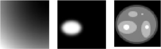

The second speed-of-sound map contains an elliptical acoustic inhomogeneity as shown in Fig. 2, which may be more common clinically. The blurred elliptical region $(2\times 1.4\mathrm{mm})$ in this map has the variable speed of sound with respect to the background. The background speed of sound was set to $1500\mathrm{m}∕\mathrm{s}$ . We were not able to compute the travel times analytically in this case for comparison.

The travel times were computed assuming that the transducers are placed on a line to the left of the phantom. These travel times were calculated using the higher-order GA approximation in 2-D using the Eqs. 20, 21, 22, 44, 45. The reference ray path was assumed to be a straight line. The line integrals over the reference ray path were evaluated numerically.

2.4.1.

Travel-time calculations

Travel times were calculated using up to fourth-order correction for different pixels for a specific transducer position. This was done in 2-D for a $50\times 50$ grid for the two specific speed-of-sound maps as shown in Fig. 2. The travel times were calculated for a 5, 10, and 15% speed-of-sound variation. The pixel size was set to $0.01\mathrm{cm}$ . The time-sampling interval was set to $33.33\mathrm{ns}$ . The transducers were assumed to lie on a line ( $z=0$ , $x⩾0$ ) to the left of the phantom, $0.01\mathrm{cm}$ apart.

2.4.2.

Image reconstruction

The images were then reconstructed iteratively using the least-squares (LS) method and conjugate gradient method. Iterative methods require the computation of system matrices. The PAT reconstruction problem can be written as¹⁶

Eq. 37

$$g=Hf,$$

where $g$ is the time-integrated pressure data, $f$ is the object function that represents the absorbed optical energy distribution, and $H$ is the system matrix. The function $g$ is defined as

$$g(x,t)\equiv \frac{4\pi }{\eta c_0}{\int }_0^{t}p(x,t^{\prime })d{t}^{\prime }.$$

We consider the 2-D geometry where the inherently 3-D OAT problem is reduced to 2-D due to the transducer’s directivity. In this case,¹⁷ for a transducer along the line $z=0$ , using the higher-order GA approximation, $g(x,t)$ can be written as

Eq. 38

$$g(x,z=0,t)=\int \int d{x}^{\prime }d{z}^{\prime }A(x^{\prime },z^{\prime })\sqrt{\frac{c(x,0)}{c(x^{\prime },z^{\prime })}}\delta [t-\tau (x,x^{\prime },z^{\prime })]\frac{c_{0}t}{\sqrt{{(x-x^{\prime })}^2+z^{\prime 2}}}.$$

The system matrix $H$ is computed by calculating the contribution of pressure signal from each pixel for a given time and transducer position. The contribution from each pixel is calculated on the basis of travel time from that pixel to a given transducer position. The system matrices were constructed in 2-D incorporating zeroth, first-, second-, third-, and fourth-order travel-time effects. The fourth-order travel-time system matrix was used for the forward model using the phantom in Fig. 2. The LS method minimizes the difference between the observed data and that obtained by projecting the object data via the system matrix. This can be written symbolically as¹⁶

Eq. 39

$$\widehat{f}=\mathrm{argmin}{\Vert g-Hf\Vert }^2.$$

Equation 39 has the solution

Eq. 40

$$\widehat{f}=H^{+}g,$$

where $H^{+}$ is the pseudo-inverse of $H$ . The iterative LS method is based on the following additive update formula:¹⁶

Eq. 41

$${\widehat{f}}^{(n+1)}={\widehat{f}}^{\left(n\right)}+\alpha \Delta f^{\left(n\right)},$$

where $\widehat{f}$ is the object estimate, $n$ is the iteration number, $\alpha$ is the step size, and $\Delta f$ is the step direction. The conjugate gradient method was used to find the new step direction. In this algorithm, the step directions are chosen so that they are conjugate to each other. This method, as outlined in Chapter 21 of Ref. 16, was used by us to perform the iterative reconstruction.

The images were then reconstructed iteratively using third-, second-, first-, and zeroth-order matrices. The image reconstruction was done on a $50\times 50$ grid with parameters as specified above. Noisy data were generated by adding Gaussian noise that was 1% of the maximum value of the noiseless fourth-order generated forward data.

3.

Results

The results below are for the specific speed-of-sound maps as shown in Figs. 2 and 2. The speed of sound in the ellipse varies with respect to the background. The line of transducers is placed to the left of the phantom along the line $x=0$ . Some of these results related to the elliptical speed-of-sound map are slightly different from those in Ref. 18. This is due to some minor improvements in the implementation of the travel-time calculations related to how accurately the slowness map is integrated over the line joining the two points.

3.1.

Relative Travel Times

In order to compare the calculated travel times with actual data, we used a speed-of-sound map that would allow for an analytical calculation of travel times. We specifically looked at the speed-of-sound map shown in Fig. 2. The relative travel times were calculated using

Eq. 42

$${\tau }_{\text{relative},\text{order}}=\frac{({\tau }_{\text{analytical}}-{\tau }_{\text{order}})}{{\tau }_{\text{analytical}}},$$

where ${\tau }_{\text{order}}$ refers to a specific-order perturbative travel time and ${\tau }_{\text{analytical}}$ is the analytically calculated travel time.

The relative travel times for the transducer at $(0,2.3\mathrm{mm})$ for phantom pixels along the line $(4.5\mathrm{mm},0)$ are shown in Fig. 3 .

Fig. 3

Relative travel times for transducer at $(0,2.3\mathrm{mm})$ for phantom pixels along the line $(4.5,0\mathrm{mm})$ for a slowly varying circular speed-of-sound map: 5, 10, and 15% variation.

From Fig. 3, we can see that even though the relative travel-time differences are small between the perturbed times and the analytical times, the second-order and higher travel times agree much more closely with the analytical times than the first-order travel time. We also observe that the higher-order travel times converge to the second-order travel times.

Figure 4 depicts the change to relative travel times for pixels located along the line $(0,1.0\mathrm{mm})$ with the transducer placed at $(0,2.3\mathrm{mm})$ in pixel coordinates for the speed-of-sound map shown in Fig. 2. The relative travel times were calculated using

Eq. 43

$${\tau }_{\text{relative},\text{order}}=\frac{({\tau }_0-{\tau }_{\text{order}})}{{\tau }_0},$$

where ${\tau }_{\text{order}}$ refers to a specific-order perturbative travel time and ${\tau }_0$ is the zeroth-order travel time. One observes that the higher-order travel-time corrections become perceivable when the speed of sound varies by 10% or more. One can also see that the travel-time perturbations seem to converge when one goes up to the fourth-order term. This suggests that one should use up to fourth-order travel-time corrections in the forward model to most accurately represent the signal.

Fig. 4

Relative travel times for transducer at $(0,2.3\mathrm{mm})$ for phantom pixels along the line $(0,1.0\mathrm{mm})$ for a specific speed-of-sound map: 5, 10, and 15% variation.

3.2.

Iteratively Reconstructed Images

Iterative image reconstruction was performed using both the speed-of-sound maps. Because the variation in speed of sound is so gradual in the circularly varying speed-of-sound map, no perceivable differences in iteratively reconstructed images could be seen between using first- and second-order system matrices. The results reported here are for the elliptical speed-of-sound map. Each group of reconstructed images use the same gray scale.

3.2.1.

Noiseless data

Figure 5 shows the iteratively reconstructed, noiseless images incorporating up to third-, second-, first-, and zeroth-order travel-time effects for the elliptical speed-of-sound map. The root-mean-square (rms) error in the reconstructed image intensities is given in Table 1 .

Fig. 5

Iteratively reconstructed images using fourth-order travel-time correction in the forward model with a 0, 1, 5, and 10% speed-of-sound variation. Images were reconstructed using various-order travel-time corrections.

Table 1

rms error in noiseless reconstructed images.

Speed of sound variation(%)	Third-order	Second-order	First-order	Zeroth-order
0	0.07202	0.07202	0.07202	0.07375
1	0.07207	0.07207	0.08195	0.25713
5	0.07514	0.07516	0.2343	0.69133
10	0.10248	0.10353	0.52213	0.74761

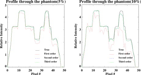
For a 1% speed-of-sound variation, there is almost no difference in images reconstructed using first-order correction and higher-order corrections. For a 5% speed-of-sound variation, the rms error in the reconstructed images are about three times smaller for higher-order reconstructions than the first-order one. For a 10% speed-of-sound variation, the images reconstructed using higher-order corrections have about a five time smaller rms error than that using the first-order one.

Figure 6 shows a line profile through the noiseless, reconstructed images at $(0,2.0\mathrm{mm})$ . One can see that the difference between higher and first-order approaches is not large for a 5% speed-of-sound variation. However, the difference is more significant for a 10% speed-of-sound variation, especially for objects lying behind the inhomogeneity.

Fig. 6

Line profile through the phantom at $(0,2.0\mathrm{mm})$ for noiseless data: 5 and 10% variation.

3.2.2.

Noisy data

Figure 7 shows the iteratively reconstructed, noisy images incorporating up to third-, second-, first-, and zeroth-order travel-time effects for the elliptical speed-of-sound map. Figure 8 shows a line profile through the noisy reconstructed images at $(0,2.0\mathrm{mm})$ . One can see that the difference between higher- and first-order approaches is again small for a 5% speed-of-sound variation. However, the difference is more significant for a 10% speed-of-sound variation especially for objects lying behind the inhomogeneity.

Fig. 7

Iteratively reconstructed images using fourth-order travel-time correction with noise in the forward model with a 0, 1, 5, and 10% speed-of-sound variation. Images were reconstructed using various-order travel-time corrections.

Fig. 8

Line profile through the phantom at $(0,2.0\mathrm{mm})$ for noisy data: 5 and 10% variation.

3.2.3.

Incorrect speed-of-sound map

To study the effect of an incorrect speed-of-sound map on higher-order GA approximation, we constructed the simulated data using the elliptical speed-of-sound map with 5.33% variation in speed of sound using the fourth-order correction. Images were iteratively reconstructing using third- and lower-order corrections assuming that the speed of variation was only 5%. Figures 9 and 10 show the reconstructed images using noiseless and noisy data, respectively. Table 2 lists the rms error in the reconstructed images using noiseless data.

Fig. 9

Images reconstructed using incorrect speed of sound map with noiseless data with the transducer placed to the left of the object along the $z$ -axi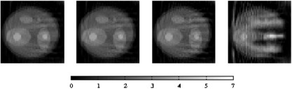s.

Fig. 10

Images reconstructed using incorrect speed-of-sound map with noisy data with the transducer placed to the left of the object along the $z$ -axis.

Table 2

rms error in noiseless, reconstructed images with a 6% incorrect speed-of-sound map.

Third-order	Second-order	First-order	Zeroth-order
0.26809	0.26809	0.31771	0.82745

In this case, the higher-order approaches still give slightly better reconstructed images when compared to the first-order approach. However, the residual artifacts in the higher-order corrections suggest that the approach is sensitive to the accuracy of the speed-of-sound map.

4.

Discussion

The higher-order GA approximation offers better results than a first-order one for a realistic speed-of-sound map that has no sharp edges with a maximum variation of $\sim 10\mathrm{\%}$ . This method is of course approximate and assumes that the speed-of-sound map is known. This method is sensitive to the accurate knowledge of the speed-of-sound map both in terms of the magnitude and the location of acoustic heterogeneity. It however does not make any assumptions about the transducer geometry. There will be certain speed-of-sound maps in practice that may result in shadow regions or caustic regions or regions where the rays get trapped. In these cases, one will not be able to correctly calculate the travel time. However, these regions will also be a problem for the GRT model using the first-order GA approximation. Hristova ¹⁰ have recently presented an application of the time-reversal algorithm to solving the photoacoustic image reconstruction problem with variable speed of sound. This is an exact approach and offers promising results but requires the detector surface to enclose the object in order to reconstruct images free from artifacts. Our higher-order GA approach could be used in those practical scenarios when the detector surface is a plane or does not completely enclose the object. It would also be useful for modeling variable speed of sound in iterative image reconstruction algorithms that are trying to model other physical factors as well in OAT.

Even though our simulations were performed in 2-D, these results should also be valid in 3-D. This is because we reduced the 3-D problem to 2-D using the 2-D directivity of the transducer, which means that the acoustic propagation is still modeled by the 3-D wave equation. We just assumed the transducer is insensitive to out-of-plane waves. In this case, the isochronous, perturbed spherical surfaces become isochronous, perturbed circles in 2-D.

5.

Conclusions

We derived a higher-order geometrical acoustics approximation to the GRT model in PAT. This incorporates the first-order correction to the pressure amplitude and higher-order correction to the travel times. We found that some differences can be seen in the travel times between higher- and first-order corrections when the speed of sound varies by 5% or more. These differences in travel times translated into the reconstructed images as well. Images that were iteratively reconstructed using the higher-order corrections were more accurate than those constructed using the first-order corrections. Similar results were obtained using noisy data, although the results were much better for the noiseless data. However, the differences between first- and higher-order models were not as pronounced when using an incorrect speed-of-sound map with $\sim 6\mathrm{\%}$ uncertainty in the magnitude of the acoustic inhomogeneity. We will conduct further studies using actual pressure data in an inhomogeneous medium in 3-D to quantify the effect of this higher-order GA approximation.