Compressed sensing in photoacoustic tomography in vivo

Zijian Guo; Changhui Li; Liang Song; Lihong V. Wang

doi:10.1117/1.3381187

1 March 2010 Compressed sensing in photoacoustic tomography in vivo

Zijian Guo, Changhui Li, Liang Song, Lihong V. Wang

Author Affiliations +

Journal of Biomedical Optics, Vol. 15, Issue 2, 021311 (March 2010). https://doi.org/10.1117/1.3381187

Abstract

The data acquisition speed in photoacoustic computed tomography (PACT) is limited by the laser repetition rate and the number of parallel ultrasound detecting channels. Reconstructing an image with fewer measurements can effectively accelerate the data acquisition and reduce the system cost. We adapt compressed sensing (CS) for the reconstruction in PACT. CS-based PACT is implemented as a nonlinear conjugate gradient descent algorithm and tested with both phantom and in vivo experiments.

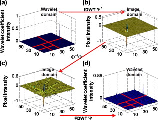
1. Introduction

The field of photoacoustic tomography (PAT) has been expanding rapidly in the past few years.¹ By combining strong optical absorption contrast and high ultrasonic resolution in a single modality, PAT can achieve much better spatial resolution at depths beyond the optical ballistic regime ( $\sim 1 mm$ in the skin) than the traditional optical modalities.^{2, 3} In PAT, biological tissues are usually irradiated by a pulsed laser. Absorbed energy is converted heat, which is further converted to a pressure rise via thermoelastic expansion. The initial pressure rise then propagates as ultrasonic waves, which are detected by ultrasound sensors, and the received ultrasonic signals are used to form an image. When the excitation laser is replaced by microwave or RF sources, the technique is called thermoacoustic tomography (TAT).^{4, 5} Both PAT and TAT have been used successfully in a variety of applications, including high-quality in vivo vascular structural imaging, hemodynamic functional imaging,^{6, 7} visualization of breast tumors,^{8, 9} and molecular imaging of biomarkers with exogenous contrast agents.^{10, 11, 12}

PAT has been implemented in various forms, and each form has its own advantages and applications.¹ In this paper, we focus on photoacoustic computed tomography (PACT, or simply PAT), in which an array of unfocused ultrasonic transducers is placed outside the object, and an inverse algorithm is used to reconstruct the image. Closed-form reconstruction formulas have been reported in both the frequency and time domains for spherical, planar, and cylindrical detecting geometries.^{13, 14, 15, 16, 17, 18, 19, 20} However, a fundamental assumption of all these algorithms is that the spatial sampling of the detecting aperture is sufficient; otherwise, undersampling artifacts, such as streaking artifacts or grating lobes, appear.

Reliable image reconstruction with sparse sampling of the detecting aperture is desirable. In practical PAT systems, it is recommended^{1, 21} to set the discrete spatial sampling period to be two to five times smaller than the sensing aperture of the detector. For a scanning PAT system, it may require hundreds or even thousands of scanning steps to acquire an image, depending on the sizes of both the detector and the detecting aperture. Such scanning usually takes several minutes to complete. To reach real-time imaging, PAT is implemented with an array of ultrasonic transducers, where all or groups of the array elements can detect photoacoustic signals simultaneously. However, the data acquisition speed is still limited by the number of parallel data acquisition (DAQ) channels, and employing a large number of DAQ channels greatly increases the system cost. For example, for a fast 512-element ring array PAT system with a 64-channel data acquisition module,²² it takes 8 laser shots to collect data from all 512 elements. For direct 3-D reconstruction PAT applications,^{23, 24} the data from a 2-D ultrasonic array is usually an extremely sparse sampling of the detecting aperture. Moreover, channel cross talk is also related to the space between neighboring elements (kerf), and an extensive spatial sampling may increase the cross talk.

Imaging an object in PAT can be understood as sensing the object in a certain domain. For example, with the Fourier-shell identity,²⁵ PAT can also be seen as detecting the spatial frequencies of the object (sensing in the Fourier domain). Sparse spatial sampling of the detection aperture implies that the spatial frequencies cannot be exactly determined. Traditional backprojection (BP) reconstruction methods¹⁶ reconstruct the image of “minimal energy” under the observation constraints. An improved reconstruction algorithm should be able to “guess” these undetermined frequency components. However, interpolation in the Fourier domain is a critical issue and usually creates artifacts in reconstructed images.²⁶ The recently developed compressed sensing (CS) theory²⁷ enables us to recover these unobserved components under certain conditions. The theory has been successfully applied in MRI,²⁸ where MRI images were able to be reconstructed from significantly undersampled K-space measurements. Reference 29 introduced the CS theory into the field of PAT, and the idea was tested in phantoms using a circular scanning PAT system. In this paper, we improve the speed of the reconstruction algorithm by adopting a nonlinear conjugate gradient descent method and demonstrate the algorithm with both phantom and animal data, using various detecting geometries.

2. Method

2.1.

Forward and Inverse Problems in PAT and Their Numerical Implementations

In PAT, pulsed laser irradiation creates pressure rises as a result of thermoelastic expansion. These initial pressure rises propagate as photoacoustic waves, which can be detected by ultrasonic sensors. Based on the pressure measurements $p (\overset{⃑}{r}, t)$ at the detecting aperture, PAT tries to reconstruct the image of the initial pressure rise distribution $p_{0} (\overset{⃑}{r})$ . The forward and inverse problems in PAT express the reciprocal relationship between $p_{0} (\overset{⃑}{r})$ and $p (\overset{⃑}{r}, t)$ . By solving the wave equation, the forward problem, which predicts $p (\overset{⃑}{r}, t)$ by $p_{0} (\overset{⃑}{r})$ , can be derived as (assuming a delta pulse heating):

Eq. 1

p (\overset{⃑}{r}, t) = \frac{\partial}{\partial t} [\frac{1}{4 π c^{3} t} \int d {\overset{⃑}{r}}^{'} p_{0} ({\overset{⃑}{r}}^{'}) δ (t - \frac{| \overset{⃑}{r} - {\overset{⃑}{r}}^{'} |}{c})],

where

c

is the speed of ultrasound, and

\overset{⃑}{r}

is the position of the ultrasonic sensor.² Sometimes, the velocity potential

φ (\overset{⃑}{r}, t) = \int_{0}^{t} p (\overset{⃑}{r}, t^{'}) d t^{'}

is employed to simplify Eq. 1:

φ (\overset{⃑}{r}, t) = \frac{1}{4 π c^{3} t} \int d {\overset{⃑}{r}}^{'} p_{0} ({\overset{⃑}{r}}^{'}) δ (t - \frac{| \overset{⃑}{r} - {\overset{⃑}{r}}^{'} |}{c}) .

The analytical inversion of Eq. 1 describes the inverse problem, which reconstructs $p_{0} (\overset{⃑}{r})$ with $p (\overset{⃑}{r}, t)$ :

Eq. 2

p_{0} (\overset{⃑}{r}) = \int_{S_{0}} {[2 p ({\overset{⃑}{r}}_{0}, \bar{t}) - 2 \bar{t} \partial p ({\overset{⃑}{r}}_{0}, \bar{t}) ∕ \partial \bar{t}] |}_{\bar{t} = | r - r_{0} |} d Ω_{0} ∕ Ω_{0},

where

\bar{t} = c t

,

S_{0}

is the detecting aperture, and

d Ω_{0} ∕ Ω_{0}

is the solid-angle weighting factor.²

To numerically model the forward and inverse problems, we need to properly discretize Eqs. 1, 2. We use a vector $x$ to represent $p_{0} (\overset{⃑}{r})$ , where each element of $x$ is the average value of initial pressure per unit volume. The size of $x$ $(N_{x} \times N_{y} \times N_{z})$ depends on the field of view (FOV) and the desired spatial resolution of the reconstructed image. We use a vector $y$ to denote the velocity potential $φ (\overset{⃑}{r}, t)$ measured by all elements of the sensor array as a function of time. The size of $y$ is the number of detecting positions $(L)$ times the number of temporal samples at each position $(M)$ . Then, the forward problem can be described as $y = Φ x$ , where matrix $Φ$ is the projection matrix. Similarly, the inverse problem can be written as $\bar{x} = Φ^{- 1} y$ , where $Φ^{- 1}$ represents the inverse process, and $\bar{x}$ is the reconstructed image.

$Φ$ and $Φ^{- 1}$ are usually extremely large matrices (each containing $N_{x} \times N_{y} \times N_{z} \times L \times M$ data points), even for 2-D reconstruction problems. For example, when reconstructing a $256 \times 256$ image with measurements from 512 detecting positions, where each position has 1024 time points, both $Φ$ and $Φ^{- 1}$ contain $3.436 \times 10^{10}$ data points ( $\sim 256 GB$ if each point is expressed in double-precision), which makes direct matrix operations computationally impractical. Reference 30 tried to solve this problem by saving only nonzero elements of metrics $Φ$ and $Φ^{- 1}$ . For each detecting element $i$ $(i = 1,2, \dots, L)$ , the forward and inverse operations are performed using a matrix of the same size as $x$ . Each element in this matrix stores an index of the temporal sample $(k = 1,2, \dots, M)$ of measurement $i$ , and this index indicates where the corresponding element of $x$ should be projected. As a result, the storage space for both the forward and inverse operations for all elements is reduced to $N_{x} \times N_{y} \times N_{z} \times L$ ( $\sim 256 MB$ for the preceding example). To fully take advantage of parallel computing capability, the responses of all the elements can be calculated simultaneously.

2.2.

Compressed Sensing for PAT

If the measurement is incomplete, matrix $Φ$ is ill-conditioned, and $Φ^{- 1}$ is obviously not an exact inversion of $Φ$ . Intuitively, an incomplete dataset usually leads to uncertainties in the recovery of the signals. In the case of PAT reconstruction with insufficient measurements, the BP method usually generates streaking artifacts or grating lobes. However, these uncertainties can be eliminated by incorporating prior information, such as sparsity constraints. The CS theory was rigorously formulated to reconstruct images from incomplete datasets. To make this possible, the CS theory relies on two principles: sparsity, which pertains to the object of interest, and incoherence, which pertains to the sensing modality. Moreover, a nonlinear reconstruction is used to enforce both sparsity of the image representation and consistency with the acquired data.

2.2.1.

Sparsity of PAT images

Unlike ultrasound imaging and all other coherent imaging technologies, PAT is devoid of speckle artifacts and sensitive to boundaries because of its optical absorption contrast.³¹ Therefore, computing the finite difference (FD) of PAT images in the spatial domain sometimes directly results in a sparse representation. When imaging objects with rich absorbing structures such as blood vessels in the mouse brain cortex, however, PAT images may not be sparse in the spatial domain. In these cases, we need to project the images onto an appropriate basis set, such as the wavelet basis. Mathematically speaking, if we use a vector $x \in R^{n}$ to represent an $n$ -pixel image and $Ψ$ to denote the wavelet basis set, then $x$ can be expanded as $x = \sum_{i = 1}^{n} a_{i} ψ_{i}$ , where $a_{i} = ⟨ x, ψ_{i} ⟩$ is the coefficient sequence of $x$ . Even when most of the image pixels have nonzero values, the wavelet coefficients may provide a concise representation of the original image: most coefficients are small, and the relatively few large coefficients capture most of the information. The speckle-free nature³¹ of PAT images further reduces the number of significant transform coefficients.

2.2.2.

Incoherence

Since the object $x$ can be visually losslessly reconstructed with only a few large transform coefficients, the problem of sensing $x$ is equivalent to capturing these large coefficients in the representation domain $Ψ$ . The forward problem of PAT can be seen as projecting the object $x$ to the sensing basis set $Φ$ , and the measurements are the resulting coefficients. The CS theory requires the two basis sets $Ψ$ and $Φ$ to be incoherent, i.e., the sensing waveforms should have a dense representation in $Ψ$ . In other words, the undersampled sensing basis $Φ$ should induce only incoherent artifacts that spread out and appear as random noise in $Ψ$ .

It is difficult to mathematically demonstrate that a physical system satisfies the incoherence condition. The transform point-spread function (TPSF)^{28, 29} was introduced to measure incoherence. Figure 1 illustrates the definition of TPSF in PAT. A wavelet transform is adopted as the sparsifying transform $Ψ$ , and we assume that a circular detecting aperture is uniformly sampled by multiple ultrasonic point sensors. The $i$ ’th transform coefficient $e_{i}$ in the domain $Ψ$ [Fig. 1] is transformed to the image space [Fig. 1] by the inverse discrete wavelet transform (IDWT). Then, the measurements are generated with the forward operator $Φ$ and transformed back to the image space [Fig. 1] with the inverse operator $Φ^{- 1}$ . Last, the reconstructed image is again transformed to the sparse domain $Ψ$ [Fig. 1] with the forward discrete wavelet transform (FDWT). TPSF can be mathematically described as $TPSF (i, j) = e_{j}^{*} Ψ Φ^{- 1} Φ Ψ^{*} e_{i}$ , and it measures the leakage of energy away from the $i$ ’th coefficient to other coefficients. The CS theory requires us to properly choose $Φ$ and $Ψ$ so that these interferences can be minimized and spread out in $Ψ$ . Readers are referred to Reference 29 for a quantitative comparison of the TPSF maps for various $Ψ$ in PAT.

Fig. 1

Illustration of the wavelet TPSF. (a) A wavelet coefficient of unit intensity; (b) IDWT of (a) in the image domain; (c) sensing (b) with 16 ultrasonic sensors and reconstructed with the BP method; and (d) FDWT of (c).

2.2.3.

Reconstruction method

If it satisfies the preceding two conditions, a sparse signal can be accurately recovered from highly incomplete datasets by solving a nonlinear convex optimization problem. We now describe in more detail the CS reconstruction method for PAT. In the CS theory, the reconstruction of image $x$ is obtained by solving the following constrained optimization problem:

Eq. 3

\min_{x} {| Ψ x |}_{1} s.t. {| Φ x - y |}_{2} < ε .

Here,

Ψ

and

Φ

are defined as earlier,

y

is the measured data, and

ε

is the parameter that controls the fidelity of the reconstruction to

y

. The parameter

ε

is usually set based on the expected noise level. The object function in Eq. 3 is the

l_{1}

norm (defined as

{| x |}_{1} = \sum | x_{i} |

). The

l_{1}

norm is used here instead of the

l_{2}

norm [defined as

{| x |}_{2} = {(\sum {| x_{i} |}^{2})}^{1 ∕ 2}

], because the

l_{2}

norm penalizes large coefficients heavily, and leads to nonsparsity. In the

l_{1}

norm, many small coefficients tend to carry a much larger penalty than a few large coefficients; therefore, small coefficients are suppressed and solutions are often sparse. In Eq. 3, minimizing the

l_{1}

norm of

Ψ x

promotes sparsity, and the constraint enforces data consistency.

The algorithm is implemented with a nonlinear conjugate gradient descent method,³² as detailed in Sec. 5. On a laptop with a dual-core $2 - GHz$ CPU and $3 - GB$ memory, the calculations usually take less than $10 \min$ using MATLAB 2008a.

3. Results and Discussions

3.1.

Tissue-Mimicking Phantom Experiment

We first demonstrate the CS method using a tissue-mimicking phantom experiment. Tissue phantoms were imaged by scanning a virtual point detector in a setup similar to that of Ref. 33 The PA source contained three black human hair crosses glued on top of optical fibers, with an interval between the hair crosses of about $10 mm$ . Laser pulses with a repetition rate of $10 Hz$ were diverged by a ground glass to achieve a relatively uniform illumination. The virtual point detectors evenly scanned the object along a horizontal circle, stopping at 240 points, and the signals were averaged over 20 times at each stop. The total data acquisition time was $8 \min$ .

Figure 2 shows the reconstruction results with the BP [Figs. 2, 2, 2, 2], the CS [Figs. 2, 2, 4, 4], and the traditional iterative³⁰ (IR) [Figs. 2, 2, 2, 2] methods, with 240, 120, 80, and 60 tomographic angles. The images are reconstructed with an FOV of $30 mm \times 15 mm$ . We can observe that the CS method is clearly superior to the BP and the IR methods. This can be shown by extracting and comparing lines from the reconstructed images [Fig. 2]. The interference level has been reduced significantly with the CS reconstruction. Moreover, as predicted by the theory, the CS scheme is robust to inaccurate measurements, so the noise level has also been suppressed. We took Fig. 2 as the gold standard, and calculated the mean-square errors (MSEs) of all other images from the standard, as shown in Fig. 2. Using the CS reconstruction method, we improved the data acquisition time in the circular scanning geometry by fourfold.

Fig. 2

Tissue phantom imaging with a virtual point detector. (a) to (d) Images reconstructed using the BP method with 240, 120, 80, and 60 tomographic angles. (e) to (h) Images reconstructed using the CS method with 240, 120, 80, and 60 tomographic angles. (i) to (l) Images reconstructed using the traditional iterative reconstruction method with 240, 120, 80, and 60 tomographic angles. (m) Lines extracted from (a), (d), (h), and (l). (n) Comparison of the mean square errors of the three reconstruction methods.

Fig. 4

In vivo imaging of the upper dorsal region of a rat with a linear array. (a) and (b) MAP images reconstructed using 48 elements with the BP and the CS methods, respectively. (c) and (d) Typical B-scans extracted from (a) and (b). (e) and (f) MAP images reconstructed using 16 elements with the BP and the CS methods, respectively. (g) and (h) Typical B-scans extracted from (e) and (f).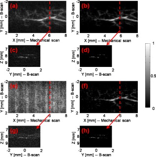

3.2.

In Vivo Experiment

The first in vivo experiment was based on a custom-designed 512-element photoacoustic tomography array system.²² The $5 - MHz$ piezocomposite transducer array was formed into a complete circular aperture. With a 64-channel data acquisition module, the system could provide full tomographic imaging at up to $8 frames ∕ s$ . We used this system to image mouse cortical blood vessels. The images were reconstructed by the BP [Figs. 3, 3, 3, 3 ] and the CS [Figs. 3, 3, 3, 3] algorithms, with 512, 256, 171, and 128 detecting elements, respectively. To achieve the optimal reconstruction results, we simultaneously used both the total variance (TV) and the wavelet as sparsifying transforms in the CS method. The undersampling artifacts appear in the outer region in Fig. 3, which is a natural result of the spatial variant PSF in PAT. Figure 3 shows the images reconstructed with 128 tomographic angles using only the TV regularization, which promotes sharp boundary features and suppresses small variances. Figure 3 shows the images reconstructed using only the wavelet regularization, and the image is “blurred.” Since 128 tomographic angles do not contain enough information to capture all the important transform coefficients, the reconstruction artifacts started to appear and some object features started to disappear. The image reconstruction result with the CS method can be further improved if a more accurate system matrix is employed. For example, unlike the virtual point detectors used in the phantom study, the detecting elements of the circular ultrasonic array system are not perfect point detectors. Therefore, further improvements can be achieved by taking into consideration of the limited detecting angles of the detecting elements.²⁵

Fig. 3

In vivo imaging of the mouse cortex with a circular ultrasonic array. (a) to (d) Images reconstructed using the BP method with 512, 256, 171, and 128 detecting elements. (e) to (h) Images reconstructed using the CS method with 512, 256, 171, and 128 detecting elements. (i) Images reconstructed using the CS method with 128 detecting elements and with only the TV regularization. (j) Images reconstructed using the CS method with 128 detecting elements and with only the wavelet regularization.

The second in vivo experiment demonstrates the capability of the CS method with linear array detecting geometry. The $30 - MHz$ broadband linear transducer array has a total of 48 elements of dimensions $82 μ m \times 2 mm$ with $100 - μ m$ pitch.³⁴ The linear array is focused in the elevation direction to perform cross-sectional (B-scan) imaging, and 3-D volume imaging can be achieved by scanning the probe in the third dimension. We scanned the upper dorsal region of a rat to image the subcutaneous vasculature and acquired a total of 166 B-scan slices. Each B-scan image was reconstructed with both the BP and the CS methods, and the Hilbert transform was taken after the reconstruction. After processing all the B-scans, the maximum amplitude projection (MAP) images were acquired through projecting the B-scans along the axial direction. Figures 4 and 4 show MAP images reconstructed with the BP and the CS methods, respectively, and one typical B-scan was extracted as shown in Figs. 4 and 4. We observed a significantly reduced noise level with the CS reconstruction. To further demonstrate the ability of the CS method in reducing the undersampling artifacts, we aggressively reconstruct the image with only 16 elements ( $1 ∕ 3$ of total 48 elements) with both the BP and the CS method. The results are shown in Figs. 4, 4, 4, 4. With the BP reconstructions, the extremely sparse linear array generates significant grating lobe artifacts. By comparison, these undersampling artifacts were effectively reduced with the CS reconstruction.

4. Conclusions

Both the phantom and the in vivo results show that the CS method can effectively reduce the undersampling artifacts. By incorporating the CS theory in the PAT reconstruction, we can effectively reduce the system cost, or cover a larger FOV with the same number of measurements. Although the CS method is demonstrated here only with 2-D problems, the generalization to 3-D reconstructions is straightforward.

Acknowledgements

This work was sponsored in part by National Institutes of Health Grant Nos. R01 EB008085, U54 CA136398, R01 CA113453901, R01 NS46214 (BRP), and R01 EB000712. L.W. has a financial interest in Microphotoacoustic, Inc., and Endra, Inc., which, however, did not support this work.

References

1.

M. H. Xu and L. H. V. Wang, “Photoacoustic imaging in biomedicine,” Rev. Sci. Instrum., 77 (4), 041011 (2006). 0034-6748 Google Scholar

2.

L. V. Wang and H. Wu, Biomedical Optics: Principles and Imaging, Wiley, Hoboken, NJ (2007). Google Scholar

3.

L. V. Wang, “Tutorial on photoacoustic microscopy and computed tomography,” IEEE J. Sel. Top. Quantum Electron., 14 (1), 171 –179 (2008). https://doi.org/10.1109/JSTQE.2007.913398 1077-260X Google Scholar

4.

R. A. Kruger, D. R. Reinecke, and G. A. Kruger, “Thermoacoustic computed tomography—technical considerations,” Med. Phys., 26 (9), 1832 –1837 (1999). https://doi.org/10.1118/1.598688 0094-2405 Google Scholar

5.

L. H. V. Wang, X. Zhao, H. Sun, and G. Ku, “Microwave-induced acoustic imaging of biological tissues,” Rev. Sci. Instrum., 70 (9), 3744 –3748 (1999). https://doi.org/10.1063/1.1149986 0034-6748 Google Scholar

6.

X. D. Wang, Y. J. Pang, G. Ku, X. Y. Xie, G. Stoica, and L. H. V. Wang, “Noninvasive laser-induced photoacoustic tomography for structural and functional in vivo imaging of the brain,” Nat. Biotechnol., 21 (7), 803 –806 (2003). https://doi.org/10.1038/nbt839 1087-0156 Google Scholar

7.

H. F. Zhang, K. Maslov, G. Stoica, and L. H. V. Wang, “Functional photoacoustic microscopy for high-resolution and noninvasive in vivo imaging,” Nat. Biotechnol., 24 (7), 848 –851 (2006). https://doi.org/10.1038/nbt1220 1087-0156 Google Scholar

8.

R. A. Kruger, H. E. Reynolds, W. Kiser, D. R. Reinecke, and G. A. Kruger, “Thermoacoustic computed tomography for breast imaging,” Radiology, 210 (2), 587 –587 (1999). 0033-8419 Google Scholar

9.

A. A. Oraevsky, E. V. Savateeva, S. V. Solomatin, A. A. Karabutov, V. G. Andreev, Z. Gatalica, T. Khamapirad, and P. M. Henrichs, “Optoacoustic imaging of blood for visualization and diagnostics of breast cancer,” Proc. SPIE, 4618 81 –94 (2002). https://doi.org/10.1117/12.469851 0277-786X Google Scholar

10.

L. Li, R. J. Zemp, G. Lungu, G. Stoica, and L. H. V. Wang, “Photoacoustic imaging of lacZ gene expression in vivo,” J. Biomed. Opt., 12 (2), 020504 (2007). https://doi.org/10.1117/1.2717531 1083-3668 Google Scholar

11.

M. L. Li, J. T. Oh, X. Y. Xie, G. Ku, W. Wang, C. Li, G. Lungu, G. Stoica, and L. V. Wang, “Simultaneous molecular and hypoxia imaging of brain tumors in vivo using spectroscopic photoacoustic tomography,” Proc. IEEE, 96 (3), 481 –489 (2008). https://doi.org/10.1109/JPROC.2007.913515 0018-9219 Google Scholar

12.

A. De La Zerda, C. Zavaleta, S. Keren, S. Vaithilingam, S. Bodapati, Z. Liu, J. Levi, B. R. Smith, T. J. Ma, O. Oralkan, Z. Cheng, X. Y. Chen, H. J. Dai, B. T. Khuri-Yakub, and S. S. Gambhir, “Carbon nanotubes as photoacoustic molecular imaging agents in living mice,” Nat. Nanotechnol., 3 (9), 557 –562 (2008). https://doi.org/10.1038/nnano.2008.231 1748-3387 Google Scholar

13.

Y. Xu, D. Z. Feng, and L. H. V. Wang, “Exact frequency-domain reconstruction for thermoacoustic tomography—I: Planar geometry,” IEEE Trans. Med. Imaging, 21 (7), 823 –828 (2002). https://doi.org/10.1109/TMI.2002.801172 0278-0062 Google Scholar

14.

Y. Xu, M. H. Xu, and L. H. V. Wang, “Exact frequency-domain reconstruction for thermoacoustic tomography—II: Cylindrical geometry,” IEEE Trans. Med. Imaging, 21 (7), 829 –833 (2002). https://doi.org/10.1109/TMI.2002.801171 0278-0062 Google Scholar

15.

M. H. Xu, Y. Xu, and L. H. V. Wang, “Time-domain reconstruction algorithms and numerical simulations for thermoacoustic tomography in various geometries,” IEEE Trans. Biomed. Eng., 50 (9), 1086 –1099 (2003). https://doi.org/10.1109/TBME.2003.816081 0018-9294 Google Scholar

16.

M. H. Xu and L. V. Wang, “Universal back-projection algorithm for photoacoustic computed tomography,” Phys. Rev. E, 75 (5), 016706 (2005). https://doi.org/10.1103/PhysRevE.71.016706 1063-651X Google Scholar

17.

D. Finch, S. K. Patch, and Rakesh, “Determining a function from its mean values over a family of spheres,” SIAM J. Math. Anal., 35 (5), 1213 –1240 (2004). https://doi.org/10.1137/S0036141002417814 0036-1410 Google Scholar

18.

R. A. Kruger, P. Y. Liu, Y. R. Fang, and C. R. Appledorn, “Photoacoustic ultrasound (Paus)—reconstruction tomography,” Med. Phys., 22 (10), 1605 –1609 (1995). https://doi.org/10.1118/1.597429 0094-2405 Google Scholar

19.

K. P. Kostli, M. Frenz, H. Bebie, and H. P. Weber, “Temporal backward projection of optoacoustic pressure transients using Fourier transform methods,” Phys. Med. Biol., 46 (7), 1863 –1872 (2001). https://doi.org/10.1088/0031-9155/46/7/309 0031-9155 Google Scholar

20.

C. G. A. Hoelen, F. F. M. de Mul, R. Pongers, and A. Dekker, “Three-dimensional photoacoustic imaging of blood vessels in tissue,” Opt. Lett., 23 (8), 648 –650 (1998). https://doi.org/10.1364/OL.23.000648 0146-9592 Google Scholar

21.

B. T. Cox, S. R. Arridge, and P. C. Beard, “Photoacoustic tomography with a limited-aperture planar sensor and a reverberant cavity,” Inverse Probl., 23 (6), S95 –S112 (2007). https://doi.org/10.1088/0266-5611/23/6/S08 0266-5611 Google Scholar

22.

J. Gamelin, A. Maurudis, A. Aguirre, F. Huang, P. Guo, L. V. Wang, and Q. Zhu, “A real-time photoacoustic tomography system for small animals,” Opt. Express, 17 (13), 10489 –10498 (2009). https://doi.org/10.1364/OE.17.010489 1094-4087 Google Scholar

23.

P. Ephrat, M. Roumeliotis, F. S. Prato, and J. J. L. Carson, “Four-dimensional photoacoustic imaging of moving targets,” Opt. Express, 16 (26), 21570 –21581 (2008). https://doi.org/10.1364/OE.16.021570 1094-4087 Google Scholar

24.

P. Ephrat, L. Keenliside, A. Seabrook, F. S. Prato, and J. J. L. Carson, “Three-dimensional photoacoustic imaging by sparsearray detection and iterative image reconstruction,” J. Biomed. Opt., 13 (5), 054052 (2008). https://doi.org/10.1117/1.2992131 1083-3668 Google Scholar

25.

M. A. Anastasio, J. Zhang, D. Modgil, and P. J. La Riviere, “Application of inverse source concepts to photoacoustic tomography,” Inverse Probl., 23 (6), S21 –S35 (2007). https://doi.org/10.1088/0266-5611/23/6/S03 0266-5611 Google Scholar

26.

M. Haltmeier, G. Zangerl, and O. Scherzer, “A reconstruction algorithm for photoacoustic imaging based on the nonuniform FFT,” IEEE Trans. Med. Imaging, 28 (11), 1727 –1735 (2009). https://doi.org/10.1109/TMI.2009.2022623 0278-0062 Google Scholar

27.

E. J. Candes, J. Romberg, and T. Tao, “Robust uncertainty principles: exact signal reconstruction from highly incomplete frequency information,” IEEE Trans. Inf. Theory, 52 (2), 489 –509 (2006). https://doi.org/10.1109/TIT.2005.862083 0018-9448 Google Scholar

28.

M. Lustig, D. Donoho, and J. M. Pauly, “Sparse MRI: the application of compressed sensing for rapid MR imaging,” Magn. Reson. Med., 58 (6), 1182 –1195 (2007). https://doi.org/10.1002/mrm.21391 0740-3194 Google Scholar

29.

J. Provost and F. Lesage, “The Application of compressed sensing for photo-acoustic tomography,” IEEE Trans. Med. Imaging, 28 (4), 585 –594 (2009). https://doi.org/10.1109/TMI.2008.2007825 0278-0062 Google Scholar

30.

G. Paltauf, J. A. Viator, S. A. Prahl, and S. L. Jacques, “Iterative reconstruction algorithm for optoacoustic imaging,” J. Acoust. Soc. Am., 112 (4), 1536 –1544 (2002). https://doi.org/10.1121/1.1501898 0001-4966 Google Scholar

31.

Z. Guo, L. Li, and L. V. Wang, “On the speckle-free nature of photoacoustic tomography,” Med. Phys., 36 (9), 4084 (2009). https://doi.org/10.1118/1.3187231 0094-2405 Google Scholar

32.

M. A. T. Figueiredo, R. D. Nowak, and S. J. Wright, “Gradient projection for sparse reconstruction: application to compressed sensing and other inverse problems,” IEEE J. Sel. Topics Signal Process., 1 (4), 586 –597 (2007). https://doi.org/10.1109/JSTSP.2007.910281 Google Scholar

33.

C. H. Li and L. V. Wang, “High-numerical-aperture-based virtual point detectors for photoacoustic tomography,” Appl. Phys. Lett., 93 (3), 033902 (2008). https://doi.org/10.1063/1.2963365 0003-6951 Google Scholar

34.

L. Song, K. Maslov, R. Bitton, K. K. Shung, and L. V. Wang, “Fast 3-D dark-field reflection-mode photoacoustic microscopy in vivo with a

30 - MHz

ultrasound linear array,” J. Biomed. Opt., 13 (5), 054028 (2008). https://doi.org/10.1117/1.2976141 1083-3668 Google Scholar

35.

E. van den Berg and M. P. Friedlander, “Probing the Pareto frontier for basis pursuit solutions,” SIAM J. Sci. Comput. (USA), 31 (2), 890 –912 (2008). https://doi.org/10.1137/080714488 1064-8275 Google Scholar

Appendices

Appendix

In this section, we describe the reconstruction algorithm for solving the constrained optimization problem in Eq. 3, which has been proved to be closely related to solving the following convex unconstrained optimization problem:³⁵

Eq. 4

\min_{x} f (x) = \frac{1}{2} {| Φ x - y |}_{2} + λ {| Ψ x |}_{1},

where

λ

is a nonnegative regularization parameter, which determines the trade-off between the data consistency and the sparsity. In order for these two problems to be equivalent,

ε

and

λ

must satisfy a special relationship. However, it is difficult to find analytical solutions if the matrix

A = Φ Ψ^{*}

is not orthogonal.³⁵ Therefore, we solved a series of

λ

to find a suboptimal solution of the problem in Eq. 3. The process is described as follows:

1. Let $λ = 0.05 {| A^{T} y |}_{\infty}$ Ref. 32, and solve problem (4) for $x$ .
2. Check the condition ${| Φ x - y |}_{2} < ε$ . If this condition holds, we increase $λ$ to promote the sparsity ${| Ψ x |}_{1}$ ; otherwise, we decrease $λ$ to enforce the data consistency ${| Φ x - y |}_{2}$ .
3. Problem (4) is solved again with the new $λ$ . Previously solved $x$ is used as the initial guess. By using this warm starting technique,³² the current optimization process takes for fewer numbers of iterations than the previous one.
4. Steps 2 and 3 are repeated multiple times.

The final solution is still only a suboptimal solution of Eq. 3. However, problem (4) can be solved with the conjugate gradient descent method with backtracking line search method,²⁸ which is computationally efficient to implement.

As mentioned in Sec. 2.1, the forward problem matrix $Φ$ is extremely large, and the direct matrix operation is computationally impractical. Therefore, the computations of both $Φ$ and its transpose $Φ^{T}$ were implemented as submodules.

Citation Download Citation

Zijian Guo, Changhui Li, Liang Song, and Lihong V. Wang "Compressed sensing in photoacoustic tomography in vivo," Journal of Biomedical Optics 15(2), 021311 (1 March 2010). https://doi.org/10.1117/1.3381187

Published: 1 March 2010

Access the abstract

JOURNAL ARTICLE
6 PAGES

DOWNLOAD PAPER SAVE TO MY LIBRARY

GET CITATION

CITATIONS

Cited by 155 scholarly publications.

Explore citations on Lens.org

RIGHTS & PERMISSIONS

Get copyright permission Get copyright permission on Copyright Marketplace

KEYWORDS

Acquisition tracking and pointing

Photoacoustic tomography

In vivo imaging

Data acquisition

Compressed sensing

Sensors

Reconstruction algorithms

1.

Introduction

2.

Method

2.1.

Forward and Inverse Problems in PAT and Their Numerical Implementations

Eq. 1

Eq. 2

2.2.

Compressed Sensing for PAT

2.2.1.

Sparsity of PAT images

2.2.2.

Incoherence

Fig. 1

2.2.3.

Reconstruction method

Eq. 3

3.

Results and Discussions

3.1.

Tissue-Mimicking Phantom Experiment

Fig. 2

Fig. 4

3.2.

In Vivo Experiment

Fig. 3

4.

Conclusions

Acknowledgements

References

Appendices

Appendix

Eq. 4

Show All Keywords

Keywords/Phrases

Search In:

Publication Years