3.1.

Confirmation of Phase Conjugation

Figure 2 shows the decay of the signal measured at the CCD in Fig. 1 as a function of sample displacement. Notably, the reconstructed signal falls off dramatically as the sample is moved, implying that we are correctly performing the phase conjugation experiment. If we examine the images captured at displacements corresponding to the red arrows in Fig. 2, we see that the bright spot shown in Fig. 2 had completely disappeared and was buried in noise in Fig. 2. This serves as confirmation that we are seeing a phase conjugate signal that is dependent on the location of scatters in the sample.

Fig. 2

(a) Reconstructed TSOPC signal measured at the CCD as the sample is displaced over $1.6\mu \mathrm{m}$ . (b) and (c) are images recorded at the locations indicated by the red arrows. This data confirms that we are measuring a phase conjugation signal that is dependent on the location of scatterers in the sample. (Color online only.)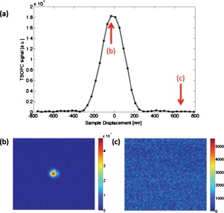

3.2.

Chicken Breast Tissue Experiments

We first examine results from chicken tissue samples of varying thickness. Figure 3 shows representative samples indicating that the thickest tissue samples used in this study were by no means transparent. Figure 3 shows the large extent of light scattering experienced by a green incident beam $(\lambda =532\mathrm{nm})$ .

Fig. 3

(a) Representative 0.25-, 0.5-, 1-, 3-, 5-, and $7\text{-}\mathrm{mm}$ -thick chicken breast sections placed above text. As the thickness increases, light scattering makes it impossible to read the text below. (b) A $3.5\text{-}\mathrm{mm}$ -diam beam of $532\text{-}\mathrm{nm}$ light scattering through a representative $7\text{-}\mathrm{mm}$ section of chicken breast tissue. For reference, the black plastic spacer is $30\times 24\mathrm{mm}$ .

We determined the scattering coefficient of the chicken breast tissue to be ${\mu }_s=30.3{\mathrm{mm}}^{-1}$ . The following data are reported as a function of the average number of scattering events experienced by a photon tracing an approximately straight path through the sample, quantified by ${\mu }_{s}L$ ( $L$ is the sample thickness). Although most photons take longer paths through the scattering material, scattering more than ${\mu }_{s}L$ times, this is a simple reference quantity for turbidity estimation. In general the ballistic, or unscattered, component of the transmission decays exponentially with depth into a scattering medium, $T_{\mathrm{ball}}=\exp (-{\mu }_{s}L)$ . All data are normalized with respect to a nonscattering sample.

The total signal contained in the reconstructed focused spot, as measured on the CCD in Fig. 1, was indicative of the amount of light that had returned to its original configuration. For simplicity, this metric can be replaced by the amplitude, or peak intensity, of the focused spot, shown explicitly in Figs. 4 and 4 . This is possible because the full width at half maximum (FWHM) of the reconstructed spot did not change as a function of scattering strength (a phenomenon that is discussed in detail later in this paper). The red curve in Fig. 4 displays the TSOPC amplitude as a function of ${\mu }_{s}L$ . Error bars correspond to the standard error from measurements made over different sample locations (i.e., different random configurations of scatterers). Although the TSOPC amplitude initially dropped off quickly, the slope began to taper off more slowly as ${\mu }_{s}L$ increased. This limited decrease is particularly noteworthy when compared to the dramatic decay of the ballistic component [blue curve, Fig. 4].

Fig. 4

(a) TSOPC amplitude (red data), ballistic transmission (blue line), total transmission (black curve), and OPC signal (green curve) as levels of scattering were increased. The square of the transmission (dashed curve) approximated the TSOPC amplitude in trend. Error bars represent the standard error over $N$ ranging from three to seven measurements. (b) TSOPC amplitude was measured as the height of the focused spot after the background signal was subtracted. (c) Signal from the $7\text{-}\mathrm{mm}$ chicken breast sample was clearly visible above the noise in the system. (Color online only.)

The signals in Fig. 4 were measured in tissue sections that ranged from $0.25\text{to}7\mathrm{mm}$ in thickness, the thickest of which corresponding to a “time reversal” of more than 200 scattering events. This is by no means trivial. Transmission through the $7\text{-}\mathrm{mm}$ tissue sample would result in a ballistic component at $-91$ on the scale shown in Fig. 4, or an attenuation of $-910\mathrm{dB}$ .

The solid black curve in Fig. 4 represents the direct transmission through the chicken breast samples measured over the collection area of the PrC, $T_{\mathrm{meas}}$ [recorded at the location denoted in Fig. 1]. The green curve shows a similar trend and represents the power that exited the PrC on playback, denoted $P_{\mathrm{OPC}}$ and recorded where indicated in Fig 1. The dependence of the TSOPC amplitude on these measured signals is discussed and modeled in Sec. 4.

3.3.

Tissue-Mimicking Phantom Experiments

To examine the dependence of our system on the angular scattering properties of the sample, we conducted experiments on tissue-mimicking phantoms composed of polystyrene spheres embedded in polyacrylamide. By varying the size of the spheres, the anisotropy factor, $g$ , of the scattering media can be altered. A measure of the angular spread of the scattered light $g$ is defined as the average cosine of the scattering angle $[g=⟨\cos \left(\theta \right)⟩]$ . Figure 5 shows the TSOPC amplitude as a function of ${\mu }_{s}L$ for four types of phantoms from highly forward scattering $(g=0.93)$ to nearly isotropic $(g=0.07)$ . We found that the more forward scattering samples resulted in a larger TSOPC signal for the same ${\mu }_{s}L$ . The solid line superimposed on the data in Fig. 5 shows the decay of the ballistic component of the transmission, while the dashed line shows the decay of the ballistic component through a sample twice as thick $\left(2L\right)$ . Except for the case of the highly forward scattering samples, the TSOPC amplitude initially decayed along the dashed line.

3.4.

Resolution Trends

To study the resolution of our TSOPC experiment, we employed a modified system in which the sample beam was focused onto the front face of the sample [Fig. 6 ]. The remainder of the system is as described in Fig. 1, and phase conjugation was used to reconstruct this spot at the front face of the sample. An imaging system formed between the lens shown in Fig. 6 and that in front of the CCD in Fig. 1 was used to relay and magnify the reconstructed spot onto the camera for detection. The spot sizes described in the following results refer to the spot size at the sample.

We found that with no scattering sample present, the measured spot was narrow in the horizontal dimension, but spread over a large range vertically [top left panel of Fig. 7 ]. However, this effect could be mitigated through the presence of strong scattering in the sample. Figure 7 shows the FWHM of the reconstructed spot in both the $x$ and $y$ directions for increasing thicknesses of chicken breast samples. Both values tapered to tight $(\sim 1.5\mu \mathrm{m})$ , nearly diffraction limited (calculated to be $1.2\mu \mathrm{m}$ ) spots, although the FWHM in the $x$ direction tapered more quickly. The same trend can be seen with tissue-mimicking phantoms in Fig. 8 .

Fig. 7

Chicken tissue samples. (a) The top left panel shows that with no sample present the reconstructed signal forms a stripe rather than a spot. The other panels show that as the scattering is increased, the stripe is reduced to a near diffraction limited spot. (b) The reduction in the size of the focused spot in the $x$ and $y$ directions. The diffraction limit in this setup was calculated to be $1.2\mu \mathrm{m}$ . Error bars represent the standard error of the FWHM made over $N=3$ measurements.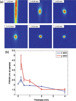

Fig. 8

Tissue-mimicking phantoms. (a) The top left panel shows that with no sample present the reconstructed signal forms a stripe rather than a spot. The other panels show that as the scattering is increased, the stripe is reduced to a near diffraction limited spot. (b) The reduction in the size of the focused spot in the $x$ and $y$ directions. The diffraction limit in this setup was calculated to be $1.2\mu \mathrm{m}$ . Error bars represent the standard error of the FWHM made over $N=3$ measurements.

4.1.

Amplitude Trends in Tissue Samples

To understand the TSOPC amplitude trend, we observed the corresponding trends for other measureable quantities in the system, including the transmission and OPC signals plotted in Fig. 4. As the thickness of the chicken sections were increased, both the transmission and OPC signal decayed in a similar manner. This shows that the power exiting the PrC on playback is proportional to the sample power entering the crystal during the recording process. Although we saw the transmission and OPC signals fall off in a similar manner, we saw a large discrepancy between these and the TSOPC amplitude (red curve). The origins of this trend will be discussed and modeled later in this section.

The signal we measured through the thickest chicken tissue sample requires additional discussion. One might expect that efficient “time reversal” would be dependent on the collection of the entire scattered wavefront. However, a measurement of the total transmission through a $7\text{-}\mathrm{mm}$ chicken breast sample over the collection area of the PrC shows that only $\sim 0.02\mathrm{\%}$ of the power incident on the sample is scattered into the collection region. This implies that at most 0.02% of the incident power is used to record the hologram for phase conjugation, and is important because it shows that the TSOPC process is capable of “time reversal” even when only a small portion of the scattered wavefront is captured. The $7\text{-}\mathrm{mm}$ thickness of chicken breast tissue does not represent a hard limitation on the capabilities of our system. It was simply the thickest sample that we measured in this study.

To cast our results in a slightly different light, consider an OCT system centered at $532\mathrm{nm}$ with $120\mathrm{dB}$ of SNR. If we tried to image these chicken samples with such a system, we would find that our depth penetration is limited by scattering to $\sim 0.5\mathrm{mm}$ , or ${\mu }_{s}L\sim 15$ . Although we are not imaging, our measured TSOPC signal through $7\mathrm{mm}$ of highly scattering tissues is noteworthy in the context of current biomedical imaging standards.

4.2.

Amplitude Trends in Tissue-Mimicking Phantoms

The amplitude signals recorded using tissues phantoms were shown to depend on the $g$ factor of the sample. This is due to the limited collection angle of the PrC. Forward scattering events were more likely to direct a photon toward the PrC, while isotropic scattering events were likely to direct a photon away from it. Thus, the final measured signal for isotropically scattering samples was less than that for forward scattering samples.

It is interesting that the measured signals in Fig. 5 fall off along the dashed line, corresponding to the ballistic component of light transmitted through a sample of double thickness. A measured TSOPC amplitude close to the dashed line implies that no advantage is gained by performing the TSOPC experiment. However, as ${\mu }_{s}L$ increased, the TSOPC amplitude began to diverge from the dashed line, meaning that we started to see an increased signal through TSOPC. The ballistic component of the scattered light was initially much stronger than the TSOPC signal, which became visible only after the ballistic component decayed significantly. In sum, Fig. 5 shows that we can efficiently collect forward scattered light, and implies that the majority of the signal we measure in tissues is related to forward directed scattering events as opposed to isotropically directed scattering events.

4.3.

Origins of Amplitude Trends

A simple predictor of the TSOPC amplitude is square of $T_{\mathrm{meas}}$ , shown as a dashed black curve in Fig. 4 and dashed curves in Fig. 5. This finding is in agreement with literature results in which phase conjugation was studied.^{11, 12} Gu and Yeh¹¹ invoked the reciprocity theorem and conservation of energy to show that under ideal circumstances (specifically in the absence of absorption and backscattering), the fidelity of the process, equivalent to our amplitude measure, scales as the square of the fraction of light intercepted by the phase conjugating device. This was experimentally verified using scattering sheets of polyprolene and polyethylene.¹² Our samples are by no means ideal, most notably in terms of nonnegligible absorption and backscattering of the tissue samples. The agreement of our TSOPC amplitude (red curve) with the square of the transmission (dashed black curve), at least in terms of trend, confirms that these predictions hold true for the case of tissue scattering as well. Our results serve to validate this theoretical prediction for a broader range of applications.

This finding deserves additional discussion. We can describe the total “time-reversed” transmission as the product of the power leaving the PrC and the transmission of the phase conjugated beam: $P_{\mathrm{TSOPC}}=T_{\mathrm{OPC}}{P}_{\mathrm{OPC}}$ . One may argue that if each photon trajectory is perfectly phase conjugated and efficiently “time reversed,” $T_{\mathrm{OPC}}$ would trend toward a value of 1, and all power directed into the sample would be effectively transmitted. The flaw in this argument is that fundamentally, our experiment cannot be described by a photon picture. If we think of the sample as a black box, and monitor only the fraction of the input light that exits one side of the box, we can make an interesting comparison. If the box contains a $50∕50$ beamsplitter (BS), we would expect 50% of the input power to exit. If we phase conjugated the exiting light, we would expect a second decrease of 50% on the way back. Although this may appear to be a very different scenario, in reality it is quite similar. In our TSOPC experiment, we can think of dividing the scattered wave into groups that have passed through channels with a particular transmission coefficient (as in Ref. 10). The bulk of the incident light is diffusely reflected, so the majority of the channels possess very small transmission coefficients. However, a small set of these channels transmits light in a fairly efficient manner. Each of these channels can be likened to a BS with a fixed transmission coefficient. When the light is phase conjugated back along these paths, they again transmit the same fraction of light. Thus, in reality, the $T_{\mathrm{OPC}}$ is equivalent to the transmission of an incident plane wave through the sample.

In our current setup, where $P_{\mathrm{OPC}}$ scales with $T_{\mathrm{meas}}$ , the preceding argument confirms the $T_{\mathrm{meas}}^2$ dependence predicted by Gu and Yeh. The amplitude of the transmitted light is the same as that expected by a double pass through the sample. The advantage, however, is that instead of the diffuse transmission that would result if a conventional mirror was used to reflect light back through the sample, we see the phase conjugate beam regain spatial coherence to reconstruct the incident light field. If a digital version of this experiment was employed, by recording the interference of the scattered field with a reference beam on a camera and playing back the phase conjugate field with a spatial light modulator, then $P_{\mathrm{OPC}}$ could be increased arbitrarily and enhanced transmission may be possible.

Although the $T_{\mathrm{meas}}^2$ curves agree with our data in trend, they do not provide a very close fit, especially for the tissue-mimicking phantom results. Although the properties of the sample are accounted for, the properties of the phase conjugation are not. In the Appendix, we formulate a model that includes both $T_{\mathrm{meas}}$ and $P_{\mathrm{OPC}}$ values to describe the crossover from ballistic to diffusive regimes. The result is as follows:

Figure 9 shows fits of this model to both the tissue [Fig. 9] and phantom data [Fig. 9]. The fits are significantly better than the $T_{\mathrm{meas}}^2$ fits for all types of samples since information about both the sample and the phase conjugation are taken into account. If we examine the $X^2$ values from fits to the phantom data [Fig. 9], we see that $X^2$ decreases with the anisotropy factor $g$ . This is attributable to the fact that the responsivity of the PrC is diminished when scatterered light enters the active area at increasing angles with respect to the incident beam. This serves to reduce the amplitude of the interference pattern written into the PrC, and results in the same outcome as the case of a PrC with optimal responsivity that shrinks in size as the $g$ factor decreases. Since tissues are highly forward scattering, we might expect that a fit to the chicken tissues sections would result in an $X^2$ similar to that of the $1\text{-}\mu \mathrm{m}$ beads. However, we found a much smaller $X^2$ value. We expect that this occurred because the chicken sections are nonideal scattering samples. The speckle pattern formed by the scattered light is not stationary due to diffusion of particles within the tissues. This implies that the particular channels that existed throughout the recording process do not necessarily exist or possess the same transmission coefficient on playback. Thus, even if a strong pattern is formed at the PrC, it may not exactly correspond to the scattering structure of the tissue on playback. A faster holographic medium or a digital implementation of this experiment may diminish this effect in the future.

Fig. 9

Model fits to (a) the experimental chicken tissue results and (b) the experimental tissues phantom results. A model that includes information about both the sample and the phase conjugation performs significantly better than the $T^2$ predictor in both cases.

4.4.

Resolution Trends

One might expect that the resolution of the TSOPC system would degrade as scattering becomes more prominent. However, we found that scattering can be beneficial in terms of resolution when a limited collection angle is employed. This experiment represented a low collection efficiency situation because the PrC was placed far from the sample plane. With no scattering sample in place, Fig. 6 shows that the sample beam had diverged significantly on reaching the PrC, and only portions of the sample beam that overlapped with the reference beam were recorded. From a Fourier optics perspective, the large-angle components of the diverging beam carried information about high spatial frequencies at the focus. Thus, by losing these components, we could no longer expect to reconstruct a diffraction-limited spot. As the sample and reference beams were orthogonally oriented in the crystal [Fig. 6], the effective recording area for the sample beam had a width of $3.5\mathrm{mm}$ (FWHM of the collimated reference beam) and length of $10.0\mathrm{mm}$ (length of the crystal). This explains the shape of the spots shown in Figs 7 and 8. Since the collection region was oblong, diverging angular components were better captured along one axis, leading to a smaller reconstructed spot along that dimension. As the samples became more highly scattering, more of the angular components were directed into the PrC, and the spot size was improved. The tapering of the FWHM to a constant value implies that beyond a scattering threshold, the angular components incident on the sample were effectively randomized such that efficient collection could be obtained over any small portion of the scattered wavefront. This finding was demonstrated previously for plastic sheet aberrators and etched glass phase screens,¹³ confirming theory and simulations on thin, random phase screen aberrators,^{14, 15} but has never been demonstrated in extended scattering samples or biological materials. Our work serves to extend these finding into the realm of realistic biological materials.

We mentioned previously in discussing our amplitude results that the peak of the detected signal was a useful metric only if the width of the spot remained constant. There were two significant differences in system geometry between the amplitude experiments and the resolution experiments described immediately above. First, the sample beam was collimated as opposed to focused on the sample. This reduced the beam divergence toward the crystal. Second, the PrC was placed as close as possible to the sample plane. Both of these geometrical factors allowed for efficient collection regardless of the level of scattering. Thus, throughout the amplitude experiments described, the FWHM of the measured spot was fixed for all measurements. Our amplitude studies showed that we could reconstruct a signal with only a small portion of the scattered wavefront, and our resolution studies provided us with evidence to claim that all relevant information was contained in this reconstruction.

4.5.

Significance and Future Work

Note that our results, in both tissues and tissue-mimicking phantoms, contrast the common misconception that light loses its coherence on scattering. While a tight pulse of light spreads as scattering occurs and spatial coherence is certainly lost, individual portions of the wavefront traveling on various trajectories through the scattering media retain relative coherence and thus are still capable of interference. We have shown a signal, dependent on coherent recording and playback mechanisms, for light that has scattered over 200 times on average. However, polarization shifts can accrue during scattering and, in the case where the scattered light is sufficiently diffuse, the light field no longer possesses a preferred polarization state. As light of an orthogonal polarization cannot interfere with the reference beam, we can expect to record at most half of the available information in this situation. We believe that future technological developments of TSOPC systems should include the capability for recording the scattered wavefront using two orthogonal polarizations, demonstrated to be useful in a related system in Ref. 10.

Although the current implementation of TSOPC has not yet been applied for imaging, diagnostics, or therapy, we envision several potentially useful applications of our technique. In the context of photodynamic therapy (PDT), it may be possible to conjugate PDT agents to strong scatterers, which can then be injected into a region to be ablated. The collected scattered light field will encode the locations of these strong scatterers, and playback (with an OPC field of increased optical power) will direct large amounts of light to the scatterer/PDT agent construct. This type of experiment would enable a clinician to target light delivery to injected agents while avoiding the remainder of the sample. Additionally, an iterative implementation of the experiment could be useful for highlighting weak absorbers buried in a scattering medium. Elastic scattering would be “time reversed” on each iteration, but absorption would occur during each pass. This could potentially enable sensitive measurements of absorbers such as glucose through a noninvasive measurement. Ideally, beyond these applications, the long-term goal of this line of research is to facilitate high-resolution deep tissue imaging.