2.1.

Optode Array Arrangements

In order to test the performance of various fNIRS optode grids for in vivo brain imaging, we created three arrangements of sources and detectors. All of the grids were first created in two dimensions with the standard interoptode spacing: $3\mathrm{cm}$ between sources and detectors in the sparse grids, and $1.3\mathrm{cm}$ for first-nearest neighbors and $3\mathrm{cm}$ for second-nearest neighbors in the high-density grid. The grids were then conformed to an $8\text{-}\mathrm{cm}$ -radius hemisphere preserving distance and angle between each optode and the center point of the grid, which was located at the apex of the hemisphere. The first array was a standard square sparse array of interleaved sources and detectors [Fig. 1 ; 7 sources and 8 detectors for 22 total measurements], which is the most commonly used fNIRS geometry.^{20, 21} The second array was a second sparse array using a line of sources flanked by two rows of detectors [Fig. 1; 8 sources and 14 detectors for 28 total measurements], which is another commonly used arrangement with the goal of increasing resolution along one axis.^{22, 23} (We will refer to this arrangement as the triangular sparse array.) The third array was a high-density grid developed for the visual cortex⁵ [Fig. 1; 24 sources and 28 detectors for 212 first- and second-nearest neighbor measurements].

Fig. 1

Diffuse optical imaging optode arrays. Sources are red squares, detectors are blue circles, and measurements are green lines. (a) Schematic of the square sparse imaging array. The two-dimensional (2-D) grid with $3\text{-}\mathrm{cm}$ spacing was conformed to an $8\text{-}\mathrm{cm}$ -radius sphere. Shown is a projection of the resulting three-dimensional (3-D) optode locations. (b) Schematic of the triangular sparse imaging array. (c) Schematic of the high-density imaging array. First-nearest neighbors have $1.3\text{-}\mathrm{cm}$ spacing and second-nearest neighbors have $3\text{-}\mathrm{cm}$ spacing. (d) Cross section through the 3-D head model. The inner brain region (yellow) has a radius of $7\mathrm{cm}$ , and the outer skin/skull region is $1\mathrm{cm}$ thick. All images shown in later figures are posterior coronal projections (direction of view noted by arrows) of a $1\text{-}\mathrm{cm}$ -thick shell around the cortical surface (dashed lines). (e) Schematic of the high-density imaging array placed over the occipital cortex of a human subject. (Color online only.)

2.2.

Forward Model

A two-layer, hemispherical head model ( $80\text{-}\mathrm{mm}$ radius) was used for forward light modeling. The model consisted of an inner brain region ( $70\text{-}\mathrm{mm}$ radius; optical properties at $750\mathrm{nm}$ : ${\mu }_a=0.15{\mathrm{cm}}^{-1}$ , ${\mu }_s^{\prime }=8.4{\mathrm{cm}}^{-1}$ ; at $850\mathrm{nm}$ : ${\mu }_a=0.17{\mathrm{cm}}^{-1}$ , ${\mu }_s^{\prime }=7.4{\mathrm{cm}}^{-1}$ ) surrounded by an outer skin/skull region ( $10\text{-}\mathrm{mm}$ thickness; optical properties at $750\mathrm{nm}$ : ${\mu }_a=0.19{\mathrm{cm}}^{-1}$ , ${\mu }_s^{\prime }=12.0{\mathrm{cm}}^{-1}$ ; at $850\mathrm{nm}$ : ${\mu }_a=0.19{\mathrm{cm}}^{-1}$ , ${\mu }_s^{\prime }=11.0{\mathrm{cm}}^{-1}$ ). These optical properties were derived by linear interpolation from the values used by Strangman ²⁴ A tetrahedral mesh (162,040 nodes) was created in NetGen. Finite-element forward light modeling was performed using NIRFAST²⁵ to generate Green’s functions for the sensitivities of each source and detector. These Green’s function were converted from the tetrahedral geometry to a voxelized space (voxels were cubic with a side length of $2\mathrm{mm}$ ) and cropped to the region with high sensitivity ( $140\text{-}\mathrm{mm}$ width, $80\text{-}\mathrm{mm}$ height, $48\text{-}\mathrm{mm}$ depth, for a total of 67,200 voxels). Sensitivity matrices, $\mathbf{A}$ , for each array were constructed using the adjoint formulation and normalized consistent with the Rytov approximation: $\mathbf{y}=\mathbf{A}\mathbf{x}$ , where $\mathbf{y}$ is a vector of differential light measurements [ $y_i=-\log (I_i∕⟨I_i⟩)$ ; where $i$ runs over all measurements], and $\mathbf{x}$ is a vector of the discrete representation of absorption perturbations in the volume.

2.3.

Inverse Formulation and Reconstruction

The finite-element model was directly inverted for image reconstruction.^{26, 27} The inverse problem minimizes the objective function: $\min \{{\Vert y_{\mathit{meas}}-\mathbf{A}\mathbf{x}\Vert }_2^2+\alpha \Vert \mathbf{I}\mathbf{x}\Vert \}$ . A solution, $\mathbf{x}={\mathbf{A}}^{\#}{\mathbf{y}}_{\mathit{meas}}$ , was obtained using a Moore-Penrose generalized inverse with, ${\mathbf{A}}^{\#}={\mathbf{A}}^T{(\mathbf{A}{\mathbf{A}}^T+{\alpha }^2\mathbf{I})}^{-1}{\mathbf{y}}_{\mathit{meas}}$ . The optimal value of $\alpha ={10}^{-2}s$ (where $s$ is the maximal singular value of $\mathbf{A}$ ) was found to provide a good balance between resolution and contrast-to-noise by evaluating in vivo activation data.⁶ The same values were used for reconstructing all three optode arrays.

2.4.

Visualization

From the resulting three-dimensional (3-D) inverted A-matrix, we selected a $10\text{-}\mathrm{mm}$ -thick cortical shell centered over the surface of the cortex (radius $65\mathrm{mm}\text{to}75\mathrm{mm}$ ). Voxels within this shell were averaged in depth to create a two-dimensional (2-D) posterior cortical projection [Fig. 1] of dimensions $140\mathrm{mm}$ by $80\mathrm{mm}$ . All reconstructions were performed using this shell. (Note that this is different from a cortically constrained reconstruction,²⁸ since the cortical region is chosen after rather than before inversion.) For visualization, we display a smaller, centered field of view of $102\text{-}\mathrm{mm}$ width and $50\text{-}\mathrm{mm}$ height in order to focus on the regions under the arrays with the highest sensitivities and lower image artifacts. This region is shown in Figs. 1, 1, 1 by the black dashed line.

2.5.

Simulation and Point-Spread Function Analysis

Point-spread functions (PSFs) were created by simulating a perturbation at a single point. The simulated absorption perturbation, ${\mathbf{x}}_{\mathbf{sim}}$ , is a vector of zeros except for one target pixel with a value of one. We then generated simulated measurements ${\mathbf{y}}_{\mathbf{sim}}=\mathbf{A}{\mathbf{x}}_{\mathbf{sim}}$ and reconstructed an image ${\mathbf{x}}_{\mathbf{recon}}={\mathbf{A}}^{\#}{\mathbf{y}}_{\mathbf{sim}}$ . With this particular choice of ${\mathbf{x}}_{\mathbf{sim}}$ , this is equivalent to examining a row from the matrix ${\mathbf{A}}^{\#}\mathbf{A}$ (known as the resolution matrix).

Since the sparse arrays often reconstruct asymmetric and elliptical responses, using the square root of the area above half maximum to construct a full width at half maximum (FWHM) tends to be a poor measure of a response’s characteristic length. Thus, we defined FWHM as the maximum separation between all pairs of points in the activation, which is a lower bound on the diameter of a circle needed to completely enclose the activation [Fig. 2 ]. Another standard image metric is the localization error, defined as the distance between the centroid of the response and the known location of the target [Fig. 2]. In neuroscience applications where the location of the activation is unknown, mislocalization and an overly large activation are both equivalent in that they cause brain hemodynamics to be measured where none actually occurred. Thus, we combined these two image metrics into a single “effective resolution” defined as the diameter of a circle centered at the known perturbation position needed to enclose the entire activation [Fig. 2], which should more closely characterize expected in vivo performance. For simplicity, all images shown were made using the $850\text{-}\mathrm{nm}$ A-matrices.

Fig. 2

Definitions of imaging metrics for point-spread function analysis shown using a simulated image reconstruction from the triangular sparse array. The target perturbation is the blue square, and the contour at half-maximum of the reconstruction is the blue line. (a) Full width at half maximum (FWHM) is defined as the maximum separation between any two points above half maximum in the reconstruction (red arrows). This is a lower bound on the diameter of a circle needed to enclose the reconstruction (red circle). (b) Localization error is the separation of the known target position and the centroid of the reconstruction (red arrows). (c) Effective resolution is the diameter of a circle centered at the known target position needed to enclose all points above half maximum in the reconstruction (red circle and arrows). (Color online only.)

Note that we do not explicitly include noise in the simulated data. However, we do set the regularization based on in vivo imaging. Thus, the reconstructed images implicitly reflect the smoothing necessary to accommodate real-world measurement noise. Working with noiseless simulated data allows us to focus the image quality evaluations on the systematic modeling and data sampling errors which are the central theme of this paper. The evaluation of image quality in the presence of noise is addressed in full with the in vivo data evaluations.

2.6.

Simulated Cortical Activations

As a bridge between point-spread functions and in vivo results, we also simulated the type of target brain activations one would expect from a retinotopic mapping study. Because each area of the visual cortex contains a map of the visual field (with adjacency preserved), moving visual stimuli create traveling waves of neuronal activity. We thus created a sequence of target activations ${\mathbf{x}}_{\mathbf{sim}}\left(\mathbf{t}\right)$ , where each frame has a target similar to the activations seen in our previous retinotopic mapping study.⁶ The visual angle mapping sequence consists of target activations $10\mathrm{mm}$ in radius traveling in an ellipse ( $20\text{-}\mathrm{mm}$ and $15\text{-}\mathrm{mm}$ major and minor axes) with a center slightly off center from the center of the field of view (from here on referred to as the elliptical target). The eccentricity mapping sequence consists of two rectangular targets ( $30\text{-}\mathrm{mm}$ width, $14\text{-}\mathrm{mm}$ height) moving upward in the field of view (to be referred to as the bar target). Reconstructed responses ${\mathbf{x}}_{\mathbf{recon}}\left(\mathbf{t}\right)$ were then constructed as earlier. Phase-encoded mapping of these periodic responses was performed as explained in below with the in vivo visual cortex data.

2.7.

Retinotopic Imaging Paradigm

The data for this analysis was acquired in a previous experiment;⁶ for this analysis, the data has been reimaged using the A-matrices described earlier. The study was approved by the Human Research Protection Office of the Washington University School of Medicine, and informed consent was obtained from all participants prior to scanning. Subjects were seated in an adjustable chair in a sound-isolated room facing a $19\text{-}\mathrm{in}$ LCD screen at a viewing distance of $90\mathrm{cm}$ . The imaging pad was placed over the occipital cortex, and the optode tips were combed through the subject’s hair. Hook-and-loop strapping around the forehead held the array in place. All stimuli were phase-encoded, black-and-white reversing logarithmic checkerboards ( $10\text{-}\mathrm{Hz}$ contrast reversal) on a 50% gray background.^{29, 30} Polar angle within the visual field was mapped using counterclockwise and clockwise rotating wedges: minimum radius $1\mathrm{deg}$ , maximum radius $8\mathrm{deg}$ , width $60\mathrm{deg}$ , and a rotation speed of $10\mathrm{deg}∕\mathrm{s}$ for a cycle of $36\mathrm{s}$ . This rotation frequency allows for each stimulated brain region to return to baseline before subsequent activations.³¹ Eccentricity within the visual field was mapped with expanding and contracting rings: minimum radius $1\mathrm{deg}$ , maximum radius $8\mathrm{deg}$ , width $1.4\mathrm{deg}$ (three checkerboard squares), and 18 positions with $2\mathrm{s}$ per position for a total cycle of $36\mathrm{s}$ . Subjects were instructed to fixate on a central crosshair for all experiments. All stimuli started with $5\mathrm{s}$ of a 50% gray screen, continued with $10\text{cycles}$ of the phase-encoded stimulus, and concluded with $15\mathrm{s}$ of a 50% gray screen.

2.8.

DOT System

Our high-density DOT instrument uses light-emitting diode (LED) sources at $750\mathrm{nm}$ and $850\mathrm{nm}$ (750-03AU and OPE5T85, Roithner Lasertechnik) and avalanche photo diode (APD, Hamamatsu C5460-01) detectors.⁵ Each detector has a dedicated $24\text{-bit}$ analog-to-digital converter (MOTU HD-192). Sources and detectors were coupled with fiber-optic bundles to a flexible imaging cap held on to the back of the head with hook-and-loop strapping [Fig. 1]. After being digitized, the APD measurements were written directly to hard disk at $96\mathrm{kHz}$ . With temporal, frequency, and spatial encoding, the system worked in continuous-wave mode with a frame rate of $10.78\mathrm{Hz}$ .

2.9.

Processing of In Vivo Data

Source-detector pair data $\left[V_i\left(t\right)\right]$ were converted to log-ratio data $[y_i\left(t\right)=-\log (V_i\left(t\right)∕⟨V⟩)]$ and bandpassed $\left(0.02\mathrm{Hz}\text{to}0.5\mathrm{Hz}\right)$ to remove long-term trends and pulse. A subset of the data corresponding to the second (triangular) sparse grid [Fig. 1] was imaged using the inverted A-matrix constructed earlier. Since the square sparse array [Fig. 1] was not a subset of the high-density array used for data collection, it was not used in the in vivo analysis. Channels with high variance $(>7.5\mathrm{\%})$ are excluded from further analysis and not included during A-matrix inversion. This data was then inverted using the high-density A-matrix constructed earlier. For both imaged data sets, hemoglobin species concentrations were determined using their extinction coefficients. As earlier, all DOT images are posterior coronal projections of a $1\text{-}\mathrm{cm}$ -thick cortical shell with the same $102\mathrm{mm}$ by $50\mathrm{mm}$ field of view. For simplicity, all images shown are $\Delta \mathrm{Hb}{\mathrm{O}}_2$ .

The phase-encoded stimuli create a traveling wave of neuronal activity along the cortical surface as the stimuli move through the visual field. Relative to the stimulus onset, each cortical position will be periodically activated with a different delay. Since we know the position of the stimulus at each time, we can match each pixel’s measured delay to the area of the visual field to which it corresponds.^{6, 32} In order to perform this analysis, the series of activations due to each stimuli (as well as the simulated cortical activation time courses corresponding to these stimuli) were down-sampled to $1\mathrm{Hz}$ (36 time points per stimulus cycle). Every pixel’s time course was Fourier transformed and the phase at the stimulation frequency $(0.0278\mathrm{Hz}=1∕36\mathrm{s})$ found. This phase then corresponds to the delay between stimulus onset and the pixel’s activation. We additionally need to correct for the finite neurovascular (hemodynamic) response time. Assuming that this lag time remains fixed at each cortical position, we correct for this delay using counterpropagating stimuli.³² Our convention is to define zero phase as the center of the visual field for the ring stimuli and as the lower vertical meridian for the wedge stimuli. Both before and after averaging, the phase maps were smoothed using a $3\text{pixel}$ by $3\text{pixel}$ moving box average.

3.1.

Point-Spread Function Simulations

First, we analyzed the point-spread functions (PSFs) for every pixel within our imaging domain (Video 1 ). Moving the target activation point sequentially through the domain showed that the dense array was able to reconstruct the response with good localization and a slightly blurred but symmetric PSF. Both sparse arrays displaced activations to the nearest area of high sensitivity (i.e., onto the line between the nearest source–detector pair). These errors can result in the reconstructed responses to multiple targets appearing either artificially far apart upon inversion [Figs. 3, 3, 3 ] or nearly identical despite large true separations [Figs. 3, 3, 3]. Additionally, while the triangular sparse array performs well in horizontal localization, it has essentially only two voxels vertically: it is binary, placing responses either above or below the center source line with no further discrimination. Both sparse arrays have multiple lines of symmetry, points that fall equidistant between two measurements. The location of activations at these points cannot be distinguished and are projected equally into the two measurements, resulting in large reconstructed responses. One particularly notable symmetry is along the source line in the triangular sparse array; a target directly beneath this line is reconstructed as a large vertical activation stretching the entire height of the pad.

Fig. 3

Representative image performance of sparse and high-density arrays. Targets are shown as red and blue squares. Half-maximum contours of the reconstructed responses are shown with the appropriately colored lines. (a) to (c) Here, two targets have been placed $4\mathrm{mm}$ apart adjacent to the horizontal midline of the arrays. The high-density array can correctly place the responses with a relatively small PSF (separation $4.4\mathrm{mm}$ ). However, the triangular sparse array artificially displaces the two reconstructions (separation $23.2\mathrm{mm}$ ) and enlarges the PSFs. The square sparse array results in reconstructions with an L-shape, which gives a large activation size, but reasonably close placement of the centroids (separation $11.5\mathrm{mm}$ ). (d) to (f) Here, two targets have been placed far apart. Although the triangular sparse array reconstructs them as superimposed (separation between centroids of only $0.6\mathrm{mm}$ ), the high-density array correctly separates them $\left(17.5\mathrm{mm}\right)$ . The square sparse array again reconstructs one of the activations in an L-shape, resulting in intermediate separation values $\left(8.2\mathrm{mm}\right)$ with a large response size. (Color online only.)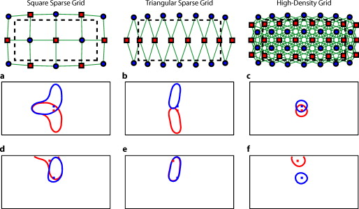

Video 1

Point-spread functions of targets placed at every location in the field of view for the sparse and high-density grids. (upper left) Simulated targets $(2\mathrm{mm}\times 2\mathrm{mm}\times 10\mathrm{mm})$ to be measured and reconstructed by the different arrays. (lower left) The response reconstructed with the high-density array. Note that the response tracks the movement of the target and that there is minimal blurring. (upper right) The response reconstructed with the square sparse array. The response jumps to the high sensitivity underneath the nearest source-detector pair, causing mislocalization and large response sizes. (lower right) The response reconstructed with the triangular sparse array. While the array can localize the target well horizontally, it has only two major positions vertically (MPEG, $19\mathrm{MB}$ ).

Image errors can be quantified using standard metrics of imaging performance (Tables 1, 2 ). The size of the reconstructed response is measured with the full effective width at half maximum (FWHM) of each target’s point-spread function [Figs. 4, 4, 4 ]. Displacement of the response from the target point is calculated using localization error [Figs. 4, 4, 4]. Since both broadening and misplacement of activations are similar in the sense that they both cause reconstructed responses where no activity should be measured, we combined resolution and localization error into a single metric of effective resolution, defined as the diameter of a circle centered at the known target location needed to enclose all activated points above half maximum [Figs. 4, 4, 4]. Judging by all three metrics, the high-density system has two advantages over the sparse arrays. First, the average image quality is higher (an improvement of $1.76\times$ in FWHM, $5.4\times$ in localization error, and $2.27\times$ in effective resolution). Second, this high performance is relatively even over the entire field of view. The performance maps of the sparse arrays alternate between areas of good and poor quality. Since most brain activations have an extent on the order of $1\mathrm{cm}$ , it is likely that sparse arrays will perform only up to the quality of their worst pixel.

Fig. 4

Image quality metrics for the point-spread functions of targets placed at every location in sparse and high-density grids. (a) to (c) Full width at half maximum of the imaging arrays. The FWHM was defined as the maximum separation of all pairs of points above half maximum contrast. For the sparse arrays, there is overall poor resolution (high FWHM) with worse resolution along lines of symmetry in the grid geometry. Also, note that the triangular array has the worst resolution directly beneath the source line, where the system cannot constrain the activation vertically. The resolution for the high-density array is high across the entire imaging domain with little variation. (d) to (f) Localization error of the imaging arrays. The localization error was defined as the separation between the known target location and the centroid of the voxels reconstructed above half-maximum contrast. While the sparse arrays have low localization error directly under measurements and along points of symmetry, between measurements, it is high. Localization error for the high-density array is uniformly low across the entire field of view. (g) to (i) Effective resolution of imaging arrays. The effective resolution was defined as the diameter of the circle centered at each target position needed to enclose the response. The sparse arrays have poor effective resolution between the measurements, and only good effective resolution directly between adjacent sources and detectors. Effective resolution for the high-density array is good across the entire imaging domain, with little variation.

Table 1

Examination of point-spread functions of sparse and dense fNIRS arrays ( mean±standard deviation).

Table 2

Performance ranges for point-spread functions of sparse and dense fNIRS arrays (minimum to maximum).

3.2.

Simulated Cortical Activations

In order to provide an intermediary evaluation between in silico point-spread functions and in vivo retinotopy experiments, which necessarily excite extended areas of cortex, we performed simulations of activations designed to approximate neuronal activation patterns seen with a retinotopic mapping experiment.⁶

In the first experiment, the target was a $1\text{-}\mathrm{cm}$ -radius circle, which moved in an elliptical pattern through the field of view [Figs. 5, 5, 5 and upper-left panel of Video 2 ]. In the second experiment, the target was a bilateral pair of rectangles moving vertically in the field of view [Figs. 6, 6, 6 and upper-left panel of Video 3 ]. A reconstructed time series was generated for both series of targets and for each of the optode arrays. The square sparse grid results in linear reconstructions along the nearest source–detector measurement [Figs. 5, 5, 5, 6, 6, 6 and upper-right panel of Videos 2 and 3]. The triangular sparse array localizes the activations well horizontally, but has only binary vertical discrimination—it can only tell whether the target is above or below the source line [Figs. 5, 5, 5, 6, 6, 6 and lower-right panel of Videos 2 and 3]. The high-density grid performs well in localizing the targets throughout both series [Figs. 5, 5, 5, 6, 6, 6 and lower-left panel of Videos 2 and 3].

Fig. 5

Simulations of activations similar to those from phase-encoded mapping of visual angle. The stimulus is of $1\text{-}\mathrm{cm}$ radius and moves in an elliptical pattern, with the center of the ellipse displaced from the center of the field of view. There are a total of 36 activations in the entire rotation series. (a) to (c) Three equally spaced frames from the sequence of targets. (d) to (f) These three activations are reconstructed with the square sparse array. The activations are displaced to the nearest measurement location. (h) to (j) Reconstructions using the triangular sparse array. The activations are located correctly horizontally, but displaced to the same vertical location. (k) to (m) Reconstructions using the high-density array. Activations are correctly placed with the correct size. (n) Legend defining the phase of the target phase-encoded stimulus. (o)The phase of each pixel’s activation at the rotation frequency using the square sparse array. This measure gives the delay between the start of the stimulus and the maximum activation of each pixel. Areas with gray have low signal-to-noise and are discarded. The square sparse array is able to correctly reconstruct the pinwheel of phase from the original stimulus, with some lobes of abnormal phases near the edges and an asymmetric shape. (p) Phase-encoded mapping using the triangular sparse array. Vertical gradients have been incorrectly reconstructed as horizontal, and some phases have been placed in the incorrect quadrant. (q) Phase mapping with the high-density array, which correctly locates all phases in the pinwheel.

Fig. 6

Simulations of activations similar to those from phase-encoded mapping of eccentricity. The stimulus is two $1.4\text{-}\mathrm{cm}$ -tall rectangles moving upward in the field of view. There are a total of 18 activations in the entire rotation series. (a) to (c) Three equally spaced frames from the sequence of targets. (d) to (f) These three activations are reconstructed with the square sparse array. The activations are displaced to the nearest measurement location, often resulting in squeezing in the horizontal direction. (h) to (j) Reconstructions using the triangular sparse array. Activations under the source planes are unconstrained vertically due to the pad’s symmetry. (k) to (m) Reconstructions using the high-density array. Activations are correctly placed with the correct size. (n) Legend defining the phase of the target phase-encoded stimulus. (o) The phase of each pixel’s activation at the rotation frequency using the square sparse array. The square sparse array is able to find the general trend of increasing phase vertically, but with many artifacts in shape. (p) Phase-encoded mapping using the triangular sparse array. Due to the inability to vertically localize activations, the array can only define two general regions of phase, and it converts gradients that should be vertical to be horizontal. (q) Phase mapping with the high-density array, which correctly locates all phases in the target.

Video 2

Simulations of activations similar to those from phase-encoded mapping of visual angle. The stimulus is of $1\mathrm{cm}$ radius and moves in an elliptical pattern, with the center of the ellipse displaced from the center of the field of view. There are a total of 36 activations in the entire rotation series. (upper left) The video of 36 targets. (lower left) Reconstructions using the high-density array. Activations are correctly placed with the correct size. (upper right) Activations reconstructed with the square sparse array. The activations are displaced to the nearest measurement location. (lower right) Reconstructions using the triangular sparse array. The activations are located correctly horizontally but jump from above the source line to below it (MPEG, $1\mathrm{MB}$ ).

Video 3

Simulations of activations similar to those from phase-encoded mapping of eccentricity. The stimulus is two $1.4\text{-}\mathrm{cm}$ -tall rectangles moving upward in the field of view. There are a total of 18 activations in the entire rotation series. (upper left) The video of 18 targets. (lower left) Reconstructions using the high-density array. Activations are correctly placed with the correct size. (upper right) Activations reconstructed with the square sparse array. The activations are displaced to the nearest measurement location, often resulting in squeezing in the horizontal direction. (lower right) Reconstructions using the triangular sparse array. Activations under the source planes are unconstrained vertically due to the pad’s symmetry (MPEG, $1\mathrm{MB}$ ).

By Fourier transforming each pixel’s time traces and finding the phases at the rotation frequency, we can perform in silico phase-encoded retinotopic mapping. By convention, zero phase of the elliptical target is defined as its most vertical position [Fig. 5] and for the bar target as the bottom of the field of view [Fig. 6]. Although the square sparse grid mislocalized many of the reconstructed targets, we see that it generates the correct pinwheel phase pattern for the elliptical target [Fig. 5, although around the edges there are some abnormalities due to the uneven sampling sensitivity] and a distorted but recognizable general phase trend from bottom to top for the bar target [Fig. 6]. To the contrary, while the triangular sparse array appeared to accurately reconstruct individual target frames, this in fact masked an inability to create a proper phase pattern for either target. With the elliptical target [Fig. 5], there are three main errors: (1) what should be vertical gradients in phase (e.g., yellow to green and blue to purple along the horizontal midline) are instead reported as horizontal gradients (in the upper field of view); (2) these gradients are reconstructed as bidirectional, resulting in local extrema of phase (yellow between two regions of green and purple between two regions of blue); and (3) in the lower field of view, the phase pattern is actually reversed, with orange appearing on the lower left and pink on the lower right. With the bar target, the triangular sparse array is unable to reconstruct the expected phase pattern [Fig. 6], again resulting in incorrect horizontal gradients and local extrema. Additionally, there is a discontinuity in phase between the lower and upper halves of the array. The high-density array is able to accurately replicate both expected phase patterns throughout the field of view [Figs. 5 and 5].

3.3.

In Vivo Activations

To complete the comparison of sparse and high-density imaging arrays, we analyzed data from our in vivo retinotopic mapping experiment⁶ using the full high-density system as well as a subset that forms the triangular sparse array. Since data was not collected with an array having the square sparse array as a subset, that array is not included in this analysis. This paradigm included four stimuli: a counterclockwise rotating wedge, a clockwise rotating wedge, an expanding ring, and a contracting ring.

Two frames from the counterclockwise wedge and expanding ring stimuli are shown in Figs. 7, 7, 8, 8 , respectively. (The entire stimuli are shown in the left frame of Videos 4 and 5 .) From previous electrophysiology, fMRI, positron emission tomography (PET), and DOT studies, we expect each wedge stimulus to produce an activation in the opposite visual cortex. From our previous DOT studies, we expect the ring stimulus to produce an activation moving upward in the field of view. While the triangular sparse array can somewhat place the wedge activations in the correct quadrant, the activations are extended and have strange shapes [Figs. 7 and 7 and upper-right frame of Video 4], often with components in the wrong quadrants. Similarly, this array often mislocalizes the ring responses or fails to reconstruct entire hemispheres of activity [Figs. 8 and 8 and the upper-right frame of Video 5]. The high-density array accurately places both activation series throughout the field of view with tighter localization [Figs. 7, 7, 8, 8 and lower-right frame of Videos 4 and 5]. We then performed retinotopic mapping using Fourier analysis, with the zero phase defined for the wedge stimulus at the stimulus directly downward [Fig. 7] and for the ring stimulus at the center of the subject’s vision [Fig. 8]. The triangular sparse array suffers the same problems in vivo that were predicted in simulation [Figs. 7 and 8; compare to Figs. 5 and 6]. The high-density array is able to accurately reconstruct the full range of phases with the correct localization for both stimuli [Figs. 7 and 8].

Fig. 7

In vivo measurement from a phase-encoded mapping study of visual angle. The stimulus is a counterclockwise rotating, counterphase flickering wedge. There are a total of 36 activations in the entire rotation series. In order to line up stimuli and activations, we used our measured $6\text{-}\mathrm{s}$ neurovascular lag. (a) and (b) Two frames from the stimulus. (c) and (d) Activations from these stimuli reconstructed with the triangular sparse array. Note the poor localization and strange activation shapes. (e) and (f) Reconstructions using the high-density array. Activations are correctly placed with reasonable sizes. (g) Legend defining the phase of the target phase-encoded stimulus. Note the $180\text{-}\mathrm{deg}$ shift from Fig. 5 due to the transfer from visual field to cortex. (h) The phase of each pixel’s activation at the rotation frequency using the triangular sparse array. Note the ability to reconstruct a pinwheel of phase. The errors are similar to those from the simulation in Fig. 5. (i) Phase mapping with the high-density array, which correctly locates all phases.

Fig. 8

In vivo measurement from a phase-encoded mapping study of visual eccentricity. The stimulus is an expanding counterphase flickering ring. There are a total of 36 activations in the entire rotation series. In order to line up stimuli and activations, we used our measured $6\text{-}\mathrm{s}$ neurovascular lag. (a) and (b) Two frames from the stimulus. (c) and (d) Activations from these stimuli reconstructed with the triangular sparse array. Note the poor localization, especially when the activation passes beneath the source line, and the inability to always locate activations in both hemispheres. (e) and (f) Reconstructions using the high-density array. Activations are correctly placed with reasonable sizes. (g) Legend defining the phase of the target phase-encoded stimulus. (h) The phase of each pixel’s activation at the rotation frequency using the triangular sparse array. Note the ability to distinguish only two regions, and the conversion of vertical gradients into horizontal gradients, similar to Fig. 6. (i) Phase mapping with the high-density array, which correctly locates all phases.

Video 4

In vivo measurement from a phase-encoded mapping study of visual angle. (left) The stimulus is a counterclockwise rotating, counterphase flickering wedge. There are a total of 36 activations in the entire rotation series. In order to line up stimuli and activations, we used our measured $6\text{-}\mathrm{s}$ neurovascular lag. Here, the stimulus is shown without flicker and at $10\times$ actual presentation speed. (upper right) Activations from these stimuli reconstructed with the triangular sparse array. Note the poor localization (especially in the lower half of the field of view) and strange activation shapes. (lower right) Reconstructions using the high-density array. Activations are correctly placed with reasonable sizes. The videos have been thresholded such that changes in hemoglobin concentration below baseline are not shown (MPEG, $1\mathrm{MB}$ ).

Video 5

In vivo measurement from a phase-encoded mapping study of visual eccentricity. (left) The stimulus is an expanding counterphase flickering ring. There are a total of 36 activations in the entire rotation series. In order to line up stimuli and activations, we used our measured $6\text{-}\mathrm{s}$ neurovascular lag. Here, the stimulus is shown without flicker and at $10\times$ actual presentation speed. (upper right) Activations from these stimuli reconstructed with the triangular sparse array. Note the poor localization, especially when the activation passes beneath the source line, and the inability to always locate activations in both hemispheres. (lower right) Reconstructions using the high-density array. Activations are correctly placed with reasonable sizes. The movies have been thresholded such that changes in hemoglobin concentration below baseline are not shown (MPEG, $1\mathrm{MB}$ ).