Arterial radius estimation from microscopic data using a new algorithm for circle parameter estimation

Han J.W. van Triest; Remco T. A. Megens; Hans C. van Assen; Bart M. ter Haar Romeny; Marc A. M. J. Van Zandvoort

doi:10.1117/1.3368679

1 March 2010 Arterial radius estimation from microscopic data using a new algorithm for circle parameter estimation

Han J.W. van Triest, Remco T. A. Megens, Hans C. van Assen, Bart M. ter Haar Romeny, Marc A. M. J. Van Zandvoort

Author Affiliations +

Journal of Biomedical Optics, Vol. 15, Issue 2, 026012 (March 2010). https://doi.org/10.1117/1.3368679

Abstract

We develop and test a new method for automatic determination of vessel wall diameters from image stacks obtained using two-photon laser scanning microscopy (TPLSM) on viable arteries in perfusion flow chambers. To this extent, a new method is proposed for estimating the parameters of a circle describing the inner diameter of the blood vessels. The new method is based on the Hough transform and the observation that three points that are not colinear uniquely define a circle. By only storing the estimated center location, the computational and memory costs of the Hough transform can be greatly reduced. We test the algorithm on 20 images and compare the result with a ground-truth established by human volunteers and a standard least-squares technique. With errors of 3 to 5%, the algorithm enables accurate estimation of the vessel diameters from image stacks containing only small parts of the vessel cross section. Combined with TPLSM imaging of anatomical vessel wall properties, potentially, the algorithm enables the correlation of structural and functional properties of large intact arteries simultaneously, without requirements for additional experiments.

1. Introduction

Due to a combination of risk factors, such as smoking, diabetes, saturated lipid-rich diets, and genetic defects, vascular disorders such as high blood pressure, atherosclerosis, and endothelial dysfunction have become symptomatic even at young ages, and are the underlying cause of over 50% of all deaths in the western world.¹

In the search for causes and potential solutions for these vascular disorders, determining luminal diameters and changes therein under the influence of pressure, flow, and/or vasodilating and vasoconstricting drugs, play an important role. Additionally, details of structural and functional changes of the vascular wall [cell density and orientation, nitrous oxide (NO) production, etc.] are potentially important parameters.

Conventional and fluorescence microscopy are often applied for the imaging of vascular structures. The information that can be acquired using these techniques, however, is mostly limited to knowledge about the structure, rather than functionality. The main cause lies in the process of preparing the tissue, as often the temperatures and chemicals involved in the preparation process severely damage the tissue.²

Recently it was shown by Megens ³ that two-photon laser scanning microscopy (TPLSM) overcomes many of these problems. Viable vessels can now be imaged after ex vivo or in vivo staining.^{4, 5} For ex vivo experiments, Megens extracted the carotid arteries and uterine arteries of mice and spanned and pressurized these between two micropipettes in a home-built perfusion chamber.

TPLSM employs two photons of half the excitation energy of the fluorophores, rather than one full-energy photon, as is used in conventional fluorescence microscopy. Therefore, excitation will occur only when the photon density is high enough, i.e., when two photons arrive at the excitable molecule at exactly the same time. The probability of excitation is thus highest in the focal area and decreases proportionally with the square of the intensity farther away. Conclusively, fluorescence effectively arises only in the volume of the focus. Furthermore, the use of near-IR photons induces less phototoxicity and photobleaching, thus keeping the tissues viable for longer periods of time. Other advantages are the increased penetration depth and absence of out-of-focus excitation, resulting in better quality images even deep within tissue, enabling high-resolution 3-D image reconstruction.

The imaging of viable tissue opens avenues for closely correlating structural and functional parameters of processes such as vascular remodeling and dynamic responses of arteries on change in flow and pressure. To quantify these latter responses, many different measures have been introduced. These measures include the wall-to-lumen ratio or the number, distribution, and orientation of cells. For many of these measures it is important to have accurate data on the vessel radius and changes therein. Radii are usually estimated by means of transmission light microscopes attached to wire or perfusion myography experiments. Within these experiments, similar mounting procedures are employed to fixate and pressurize vessels to enforce circular cross sections. However, with the ability of high-resolution 3-D imaging viable arteries, new opportunities arise such as integrated subcellular imaging combined with local perfusion myography. Potential application of these opportunities can be found in the study of the causes of vascular disorders as well as testing and understanding of vessel-diameter modifying drugs.

Estimating the radius of a vessel from TPLSM data is far from trivial. To achieve subcellular resolution, mostly high magnifications in combination with additional optical zoom are applied, resulting in a small field of view of typically $100 \times 100 μ m$ . As a result, only a shallow arc of the wall is imaged, severely complicating the accurate estimation of the vessel diameter. Furthermore, the noisy, anisotropic nature of the data causes edges to be poorly defined, making it hard to localize the exact position of the vessel wall boundaries. In this paper, a new algorithm is introduced based on the Hough transform and on work by Chan ⁶

The main point of innovation introduced in this paper is a tool to study the dimensions of the structures within blood vessels. As modality, we use TPLSM, which, as opposed to conventional fluorescence microscopy, can image biological tissue under physiological conditions. This enables the study of both structural and functional parameters, such that it is no longer necessary to perform separate experiments for myography and structural studies, thus saving valuable time and resources. At the same time, the resulting images are a better representation of the tissue under physiological conditions, and as such the extracted parameters can become more relevant.

In the remainder of this paper, a brief overview of existing methods that can be employed for the estimation of the diameter of blood vessels is given, and a new method is introduced. Then, this new algorithm is evaluated by means of experiments and compared with a commonly used method. The paper is finalized with a discussion and conclusion on the proposed algorithm.

2. Methods

2.1.

Methods for Automatic Radius Estimation

Using TPLSM to image viable blood vessels, two types of recordings are frequently made, either a $z$ stack consisting of a number of $x y$ images, or an $x z$ slice. A $z$ stack contains a volume of image data [see Fig. 1 ], whereas an $x z$ slice is a single cross-sectional image perpendicular to the long axis of the vessel [see Fig. 1]. Generally, in a $z$ stack, a larger $z$ step (i.e., a lower $z$ resolution) is used than in a single $x z$ image. This increased $z$ step size is needed to shorten the recording time, thus reducing damaging factors such as tissue heating and photobleaching.

Fig. 1

Two types of data sets are commonly recorded. (a) $z$ stack represented by the cube intersecting with the vessel. Note the definition of the axes. The $x$ and $z$ axes are defined as perpendicular to the axis of the vessel, whereas, the $y$ axis is parallel to this axis. (b) $x z$ slice. For the sake of clarity, the previous definition of axes is preserved for the 2-D images. (c) Example of a murine uterine data set (contrast inverted).

When vessels are mounted and pressurized between two micropipettes,³ it is assumed that the cross section of the vessel becomes a circle [see Fig. 1]. This assumption is also employed in regular perfusion myography experiments and is both realistic and helpful. One should consider that the vessels under study are not calcified, have no plaque and are essentially a tube with an elastic wall under pressure. Large amounts of 3-D multiphoton images of small and large, elastic and muscular arteries confirm the circular shape of mounted and pressurized arteries. As an example, we refer to various previous publications, (e.g., Refs. 3, 4). Under this assumption, estimating the radius of the vessel now boils down to fitting a circle to the edge of the blood vessel-lumen boundary, without the requirement for additional shape detection. The task of fitting circles to (noisy) data is a thoroughly studied subject in many fields of science.^{7, 8} In general, two groups of methods can be distinguished, namely, statistical methods and Hough-transform-based methods. Next, the two groups of methods are briefly described, after which our new method is proposed.

2.1.1.

Statistical methods

Statistical methods seek to minimize a certain criterion or cost function, that expresses the accuracy of the fit. According to Chan, ⁶ roughly speaking, there are two variations of the cost function for fitting a circle to a set of points. The first cost function is based on the sum of the geometric distances of points to the fit (the geometric cost function), whereas the second is based on the minimization of difference in areas of the circles caused by each data point (algebraic cost function).

A circle can be described using

Eq. 1

{(x - x_{c})}^{2} + {(y - y_{c})}^{2} = r^{2},

in which

x_{c}

and

y_{c}

form the center coordinate of the circle, and

r

is the radius. Cost functions based on geometrical distances are of the form:

Eq. 2

J_{gd} = \sum_{i} {{[{(x_{i} - \hat{x})}^{2} + {(y_{i} - \hat{y})}^{2}]}^{1 ∕ 2} - \hat{r}}^{2},

in which

(x_{i}, y_{i})

is the

i

’th data point,

(\hat{x}, \hat{y})

is the estimated center, and

\hat{r}

represents the estimated radius of the circle. Algebraic cost functions, i.e., cost functions based on minimization of the difference in areas, are based on

Eq. 3

\frac{J_{a}}{π^{2}} = \sum_{i} {[{(x_{i} - \hat{x})}^{2} + {(y_{i} - \hat{y})}^{2} - {\hat{r}}^{2}]}^{2} .

The fitting procedure aims at minimizing the cost function $J_{a}$ or $J_{gd}$ . The method for minimizing $J_{gd}$ is dubbed the full least-squares method by Umbach and Jones⁹ and yields unbiased solutions. A clear disadvantage of the geometrical cost function, however, is the lack of a closed-form solution, and therefore, nonlinear techniques must be used to find a solution. These nonlinear techniques, however, are known to be sensitive to the initial conditions, have tendencies to converge to local minima, or are slow to converge in general.

Minimizing the algebraic cost function $J_{a}$ , on the other hand, does yield a closed-form solution. One of the methods employing the algebraic cost function is referred to as the Kåsa method^{8, 9} and is by far the most widely used method.⁷ A disadvantage of this method, however, is that the results are biased when the data points are not symmetrically distributed over the edge.⁸ Furthermore, it has been shown by Thomas and Chan¹⁰ that when the arc length becomes smaller and/or the noise becomes higher, the bias increases. Last, due to its least-squares nature, the method is highly sensitive to outliers. For the derivation of the closed-form solution of the Kåsa estimator see Refs. 8, 10.

2.1.2.

Hough transform

A fundamentally different concept is employed by the Hough transform (HT). The HT was first proposed in 1962 by Hough¹¹ and used for, among others, the recognition of patterns in bubble chambers. The basic idea of the HT is that detecting a peak in parameter space is a much easier task than the identification of a complex shape in image space.¹²

The HT for lines considers a set of $N$ image points $(x_{i}, z_{i})$ with $i ∊ {1 \dots N}$ located on a straight line [see Fig. 2 ]. The general parametrization of an arbitrary line is given by

Eq. 4

z = \hat{m} x + \hat{c},

in which

x

and

z

are coordinates in image space, and

\hat{m}

and

\hat{c}

are the estimated slope and intersect, respectively. Each point

(x_{i}, z_{i})

can be part of an infinite number of lines, parameterized by combinations of

\hat{m}

and

\hat{c}

. The relation between

\hat{m}

and

\hat{c}

describes a straight line, which is formulated by

Eq. 5

\hat{c} = - x_{i} \hat{m} + z_{i} .

Fig. 2

Basis of the HT for line detection: (a) $(x, z)$ points in image space; (b) $(m, c)$ parameter space, where the label of each line corresponds with the label of each point in (a); and (c) 3-D representation of the discrete accumulator array corresponding to (b). The location of the peak in the array represents a small range of parameters that best describe the line in (a).

The space described by $\hat{m}$ and $\hat{c}$ is called the parameter space. Each point in the image can thus be described by a line in parameter space [see Fig. 2]. The process of describing each point in image space by a line in the parameter space is called back projection.

The parameter space can now be sampled, resulting in a discrete array, called accumulator array. Within the array, each bin represents a small range of the parameters $\hat{m}$ and $\hat{c}$ . Each time a line describing a set of parameters traverses a bin within the array, its value is incremented. The set of parameters representing the line in the original image can now best be found by searching for the highest value in the accumulator array.

The coarseness of the discrete parameter space requires some extra attention, since each bin represents a range of values rather than a single point in parameter space. For higher precision, smaller bins are required, but the drawback of these smaller bins is that a peak might be smeared out over multiple bins, and therefore is lost in the background noise.

The HT can easily be extended to find any parameterizable shape. The parameter space will then have equal dimensionality as the number of parameters necessary to describe the very shape. As we are trying to fit a circle to a set of noisy points, for a normal circular HT, we need a 3-D parameter space, with its axes on the $x$ and $z$ coordinates of the center and the radius $r$ of the circle¹² [see Eq. 1]. Now each point in the image space is represented by a cone in parameter space with its top point at $(x_{i}, z_{i}, 0)$ . Each point $(x, z, r)$ in parameter space represents a circle with radius $r$ centered at $(x, z)$ . Now, finding the circle that best fits a circular set of data points boils down to finding the maximum in the corresponding 3-D accumulator array.

The HT has many attractive properties. The transform is very robust to the presence of random noise, since single (noise) pixels will give rise only to marginal background hits in parameter space, and will therefore not influence the peak detection. In addition, by looking for peaks in the accumulator array partly occluded or slightly distorted objects can be detected as well. Furthermore, multiple instances of an object can easily be detected by looking for multiple peaks. Finally, the character of the HT makes it possible to be implemented in a parallel fashion, giving rise to real-time detection algorithms. In addition to these positive properties, however, it has one major drawback. The computational and storage burdens of the HT are high, and rise exponentially with the number of parameters. For example, when an object with $q$ parameters is to be found using $α$ bins per parameter in accumulator space, the storage will be¹² as high as $α^{q}$ . A large part of the computational load is caused by the storing and filling of the accumulator array. For each point that is being processed in image space, all bins in parameter space that can represent this point in the image must be found and incremented, resulting in a large computational burden. The three parameters used by the traditional HT for circles, combined with the need for high accuracy, will render this computational burden prohibitively large.

2.1.3.

Proposed algorithm: a modified HT

To reduce the computational burden, in this paper a new algorithm for the estimation of the radius and center of a circle is proposed. It is based on the HT and the work of Chan ⁶ on statistical estimators. The algorithm seeks to combine the robustness against noise of the HT and the efficiency of the work of Chan in one algorithm. By employing the fact that any set of three noncollinear points uniquely define a circle, we can reduce the dimensionality of the accumulator array. For each set of three points from the detected edge points, the corresponding circle-center is calculated, which votes for the center of the vessel.

As mentioned by Chan, ⁶ a set of three points that are not collinear define an unique circle. Thus, using Eq. 1 and three random sample points, $x_{i}$ and $z_{i}$ , from the data, a system of three equations can be formed:

Eq. 6

{\begin{matrix} {(x_{1} - x_{c})}^{2} + {(z_{1} - z_{c})}^{2} = r^{2} \\ {(x_{2} - x_{c})}^{2} + {(z_{2} - z_{c})}^{2} = r^{2} \\ {(x_{3} - x_{c})}^{2} + {(z_{3} - z_{c})}^{2} = r^{2} . \end{matrix}

By subtracting the first equation from the second and the third, and after some rearranging, the following set of equations emerges:

Eq. 7

[\begin{matrix} 2 (x_{2} - x_{1}) & 2 (z_{2} - z_{1}) \\ 2 (x_{3} - x_{1}) & 2 (z_{3} - z_{1}) \end{matrix}] (\begin{matrix} x_{c} \\ z_{c} \end{matrix}) = (\begin{matrix} x_{2}^{2} + z_{2}^{2} - x_{1}^{2} - z_{1}^{2} \\ x_{3}^{2} + z_{3}^{2} - x_{1}^{2} - z_{1}^{2} \end{matrix}) .

Solving this equation for

(x_{c}, z_{c})

results in

Eq. 8

(\begin{matrix} x_{c} \\ z_{c} \end{matrix}) = A^{- 1} b,

in which

A

and

b

are

Eq. 9

A = 2 (\begin{matrix} x_{2} - x_{1} & z_{2} - z_{1} \\ x_{3} - x_{1} & z_{3} - z_{1} \end{matrix}),

Eq. 10

b = (\begin{matrix} x_{2}^{2} + z_{2}^{2} - (x_{1}^{2} + z_{1}^{2}) \\ x_{3}^{2} + z_{3}^{2} - (x_{1}^{2} + z_{1}^{2}) \end{matrix}) .

Using this result, it is possible to generate estimates for the circle center defined by each combination of three points. In total, for a set of $N$ points, this will give rise to $N! ∕ [3! (N - 3)!]$ unique estimations of sets of parameters, each set defining a single point in parameter space. In contrast to the traditional circular HT, which must find and update all points on a cone, we propose to increment only a single bin that represents the set of parameters resulting from Eq. 8.

In the proposed algorithm, a 2-D accumulator array is used to create a histogram of possible centers. Each triplet of edge points votes for a possible center of the circle describing the edge of the vessel, and is stored by incrementing the corresponding bin in the accumulator array.

After peak detection, the most likely center of the circle that represents the cross section of the vessel is found. Using a second voting mechanism, which uses a 1-D accumulator array, the radius is estimated. For each edge point $x_{i} = {x_{i}, z_{i}}$ , the distance to the center $x_{c} = {x_{c}, z_{c}}$ is calculated. This is done by calculating

Eq. 11

r_{i} = ‖ x_{i} - x_{c} ‖ = {[{(x_{i} - x_{c})}^{2} + {(z_{i} - z_{c})}^{2}]}^{1 ∕ 2} .

Each $r_{i}$ votes for a certain radius. The value for the radius that is voted for most is considered the estimated radius of the vessel. The advantage of this approach is that when the points on the edge are from multiple layers of the vessel wall, the influence of faulty estimations on the estimation of the radius will be limited.

Three points of consideration require special attention. The first is the size of the bins. The bins in the accumulator space should not be too large, as the resolution of the estimation will deteriorate. On the other hand, bins that are too small will fail to combine evidence of the center that is the most likely candidate for the fit. In the worst case, each bin contains only one vote, therefore lacking a definite peak. To combine both accuracy and robustness, it is chosen to estimate the coordinates of the center and the radius at an accuracy of $1 pixel$ . Effectively, the resolution for the localization of the center of the circle will be of the order of the size of $1 pixel$ .

Second, as we can see, the larger the distances between the three points used for the estimations, the smaller the influence of noise will be on the result. For this reason, the vote is modified by a weight. The weight is calculated by the average distance between the points used for the estimation. The weight is given by

Eq. 12

w_{i} = \frac{1}{3} (‖ x_{1} - x_{2} ‖ + ‖ x_{1} - x_{3} ‖ + ‖ x_{2} - x_{3} ‖),

in which

x_{1}

,

x_{2}

, and

x_{3}

are the three edge points that are involved in the estimation.

Last, the number of points that form the set of edge points must be considered. The traditional HT for circles will generate a cone for each point in the image, therefore guaranteeing peaks caused by the intersections of these cones. In the proposed algorithm, however, each set of three edge points will give rise to one single point in the accumulator array. Therefore, there must be enough points available to give enough hits for a peak to form. On the other hand, together with the number of points in the data set, the execution time will rise exponentially. During the experiments, the number of points will be varied to acquire a minimum number of points for reliable results.

2.1.4.

Finding the edge points

As input to the algorithm, a set of points on the edge of the vessel wall must be selected. Only points on the luminal sides are selected as, in general, this edge is smoother. The outer diameter, together with the diameters of other structures in the vessel, can then manually be found by changing the diameter of a second circle centered at the same center as the inner circle.

When acquiring the set of points, some difficulties arise with the uneven intensities within the image. As we can see in Fig. 3 , the intensities of the points on the far side of the vessel wall are greatly reduced. This especially holds for points for which the light must traverse a dense optical path, and can be attributed to the scattering of the photons along this inhomogeneous optical path.¹³ Since the reduction of the intensity is position-variant, classical approaches such as deconvolution cannot be used to compensate for the lost intensity.

Fig. 3

Demonstration of the scattering due to thick layers of tissue (inverted contrast). Since the fluorescent photons must travel through a large inhomogeneous optical system, many photons are scattered. Arrows denote the regions that are affected most by the scattering. Furthermore, note the highly anisotropic blurring that occurs in the $z$ direction, due to the point spread function of the optical system. Image adapted from Megens ³

To overcome this problem, we decided to make the localization of the edge points dependent on the path traversed by the recorded photons. In other words, edge points are found by scanning vertical lines over the image and thresholding these lines at a value that is a fraction $α$ of the maximum $I_{m}$ on that line. The value of $α$ can now be modified to find the best set of points. Initial experiments indicate that a value for $α = 0.3 - 0.5$ gives best results.

The method of constructing the edge point set can now be summarized as

1. Find the horizontal line that has the largest part of the line in common with the lumen of the vessel.
2. For each point on this line;
- a. Extract the pixel values on a vertical line through the point toward the vessel wall.
- b. Determine the maximum intensity $I_{m}$ on the line.
- c. Find the coordinate of the first point to have an intensity higher than $α \times I_{m}$ , and store this.

When points are required on both sides of the vessel lumen, the horizontal line is positioned such that it will separate the vessel roughly into two equal hemicircles, and lines are traced in both directions toward the vessel wall.

2.2.

Experimental Protocols

2.2.1.

Acquisition of data sets

The data sets used in this study were acquired for the study as described by Megens ³ Carotid (elastic) and uterine (muscular) arteries from $12 - to 20 -week$ -old C57Bl6/J mice were excised and stained using, among others, eosin. Eosin is a strong and specific fluorescent marker for elastin, which can be found in the elastic laminae within the vessel wall. The arteries were imaged using a standard BioRAD 2100 MP multiphoton system, applying $140 - fs$ pulsed Ti:sapphire laser tuned at $800 nm$ as the excitation source. For more details, see Ref. 3 on the exact labeling, mounting, and imaging procedures.

2.2.2.

Implementation of the algorithm

The algorithm was implemented using C++. Using a graphical user interface (see Fig. 4 ), the user can select an image, from both $z$ stacks and $x z$ scans, and perform simple image-processing techniques to the image, such as resampling, noise reduction, and histogram modifications. When processing $z$ stack recordings, a single $x z$ slice is to be extracted from the volume, which can be selected by moving the appropriate sliders. Furthermore, before estimation, the parameters for selection of the edge points can be modified.

Fig. 4

Main dialog of the tool. After estimation, it gives the user the opportunity to manually modify the estimate. Furthermore, a second circle, centered in the estimated circle center, can now be used to estimate the vessel wall thickness.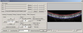

After the estimation process, the interface offers the possibility to measure the thicknesses of other structures within the vessel wall by modifying a second circle around the same estimated center. This option further extends the usefulness of the proposed method as it now becomes feasible to quantitatively study the structure while keeping the vessels viable, as opposed to conventional fluorescence microscopy.

2.2.3.

Evaluation of the algorithm

Results of the proposed algorithm are compared both with a ground truth, established by five human observers, and with the Kåsa method (see Sec. 2.1.1). The latter will from now on be referred to as the least-squares estimator (LSE).

For the evaluation of the algorithm, 10 $x z$ scans and 10 $x z$ slices from two $z$ stacks were selected. The data sets were chosen to be representative of the images commonly acquired. The images were converted to gray scale by means of taking the average of the color channels in each of the pixels. The images were then resampled to an isotropic grid, with pixel sizes of $0.5 \times 0.5 μ m$ , by means of bilinear interpolation. No noise-reduction techniques were applied to reduce the influence of these techniques on the location of the edge, and test the performance of the algorithms under noisy conditions.

Since no prior knowledge on the diameters of the lumen was available, only sets were chosen, showing the vessel wall on both sides of the lumen. From this, a ground truth was derived manually by five volunteers. To randomize the influence of display settings, the volunteers performed the manual estimations both on a CRT and an LCD screen. The manual determination was performed using a tool that is implemented in the program. The volunteers were asked to position two blue lines on both the upper and lower side of the lumen (see Fig. 5 ). By pressing the Snapshot button, the distance between the two lines was measured and stored. No significant difference between the results acquired on a CRT monitor and those acquired on an LCD screen was found. The average of all manual estimations for each of the images is considered as the ground truth. Table 1 shows the standard deviation of the manual estimations, which roughly correspond with $4 pixels$ or $2 μ m$ . From these results, we can conclude that the determination of the inner radius of a blood vessel is slightly more difficult for slices extracted from $z$ stacks. The lower accuracy is due to the diminished resolution of the $z$ stacks, making the edges less pronounced.

Fig. 5

Tool to manually estimate the radius of a vessel in an image that shows both the upper and the lower vessel wall.

Table 1

Standard deviation of the manual estimations by the volunteers, expressed in percents of the total radius.

Slice Type	Standard Deviation of Estimations
$x z$ scans	0.7%
$z$ stack slices	1.1%

The estimations were made both by using the proposed algorithm and by LSE. For a description of the LSE algorithm, see Refs. 8, 10.

The number of edge points used during the estimations is varied from 50 to 150 in steps of 10. The value for $α$ necessary to determine the edge points is set to 0.40. The estimations are performed while taking into account both one and two sides of the vessel. In the case of using the single edge, we use the top edge, which is defined as the luminal side of the wall that is nearest to the optical system.

Typically, scans show only a small part of the vessel wall that is nearest to the optical system. The part visible in a recording represents an angle at around $π ∕ 4$ of the cross section. To simulate these conditions, edge points are extracted from the vessel wall such that the angle of the arc they describe is around $π ∕ 4$ . The range from which the edge points are selected to represent this angle is calculated using the ground truth acquired as already described.

Each estimate is compared to the ground truth, and the difference is expressed in percents according to $(E_{e} - E_{g}) ∕ E_{g} \times 100 %$ , where $E_{e}$ is the estimated value for the inner radius, and $E_{g}$ is the ground truth.

3. Results

3.1.

Number of Points Required for Accurate Estimations

Figure 6 shows the errors for both algorithms on the $x z$ slices, while both sides of the lumen were taken into account. We can conclude that for the proposed method, the number of points required to achieve accurate results should be higher than 100. The higher number of points necessary for accurate estimates can be explained by the fact that for these shallow arcs, the peak within parameter space is more smeared out, and therefore more sensitive to noise. Furthermore, LSE shows poor accuracy and high standard deviations of error. The lack of accuracy in these fits can be attributed to inherent LSE sensitivity to outliers in the set of data points. The outliers originate from the noisy character of the data, leading to unusable radius estimations.

Fig. 6

Errors of the proposed algorithm (red lines) and LSE (blue lines) against the number of points for the $x z$ slices while both sides of the edges are visible: (a) the average error from all 10 slides against the number of points in the set of edge points and (b) the standard deviation of these errors. The graphs indicate that for the proposed algorithm, at least 100 points are required, whereas for LSE, the number of points on the edge does not seem to make a difference. (Color online only.)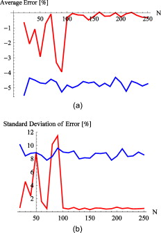

As mentioned, selecting a suitable number of points for the proposed method is a trade-off between execution costs and accuracy. The LSE on the other hand, does not depend on the number of data points. For this reason, the required number of edge points is estimated to be between 100 and 150. These values are used in the following.

3.2.

Estimations Using Both Edges

Table 2 summarizes the results acquired for both algorithms when taking into account the edges at both sides of the lumen. The results concerning the $x z$ scans show that the proposed method has errors in the range of $- 0.2 \pm 0.5 %$ , which corresponds with roughly $- 1 \pm 2 pixels$ on a diameter of $440 pixels$ . This is in contrast with the results obtained using the LSE, which gives rise to errors in the magnitude of $- 4.8 \pm 8.5 %$ , corresponding to roughly $- 20 \pm 40 pixels$ on a diameter of $440 pixels$ .

Table 2

Percentual errors for double-edged images of the new algorithm (PM) and the LSE with respect to the ground truth.

No.pts.	Double Edge, xz scan		Double Edge, z stack
No.pts.	PM (%)	LSE (%)	PM (%)	LSE (%)
100	$- 0.30 \pm 0.58$	$- 4.82 \pm 9.00$	$0.51 \pm 0.53$	$0.28 \pm 0.49$
110	$- 0.03 \pm 0.43$	$- 5.00 \pm 8.89$	$0.60 \pm 0.43$	$0.15 \pm 0.64$
120	$- 0.13 \pm 0.67$	$- 4.86 \pm 9.16$	$0.42 \pm 0.49$	$0.19 \pm 0.61$
130	$- 0.15 \pm 0.34$	$- 4.58 \pm 7.98$	$0.33 \pm 0.61$	$0.19 \pm 0.55$
140	$- 0.47 \pm 0.57$	$- 4.68 \pm 8.14$	$0.37 \pm 0.69$	$0.23 \pm 0.47$
150	$- 0.21 \pm 0.34$	$- 4.61 \pm 8.09$	$0.23 \pm 0.56$	$0.14 \pm 0.60$

The first column represents the number of points used in the estimations. PM signifies the proposed method, whereas LSE represents the Kåsa method. Errors are given in the form of mean±standard deviation. The two main columns represent double edge in xz slices and double edge in xz slices derived from z stacks, respectively.

For the estimations of the diameters performed on the slices taken from the $z$ stacks, both algorithms performed similarly ( $0.4 \pm 0.5 %$ for PM versus $0.2 \pm 0.6 %$ for the LSE method). This difference is due to the fact that the resampling procedure used inherently will reduce the effect of random noise. By having a lower noise level in the image, the extracted set of data points will be more coherent, and therefore, there will not be many outliers. Outliers are an important cause of poor results in least-squares-based methods.

3.3.

Estimations Using a Single Edge

In Table 3 , the errors of the estimations for both $x z$ scans and $z$ stack slices are given while extracting the edge points only from the side nearest to the optical system. Since only one edge was used to find the set of edge points, less information is available on the position of the $z$ coordinate of the circle center. This gives rise to significantly higher errors and uncertainties. We can conclude that for the $x z$ scans, the proposed method (errors in the range $- 3.1 \pm 2.2 %$ ), outperforms the LSE method (errors in the range $- 7.2 \pm 14.3 %$ ).

Table 3

Percentual errors for single-edged images of the new algorithm and the LSE with respect to the ground truth.

No.Pts.	Single Edge, xz scan		Single Edge, z stack
No.Pts.	PM (%)	LSE (%)	PM (%)	LSE (%)
100	$- 3.48 \pm 2.25$	$- 7.17 \pm 12.66$	$1.31 \pm 9.57$	$4.71 \pm 5.97$
110	$- 3.23 \pm 2.70$	$- 5.31 \pm 14.23$	$3.69 \pm 10.78$	$4.38 \pm 5.72$
120	$- 3.26 \pm 2.03$	$- 6.14 \pm 15.20$	$2.91 \pm 5.93$	$4.53 \pm 5.90$
130	$- 3.12 \pm 1.97$	$- 9.46 \pm 13.35$	$4.18 \pm 7.15$	$4.85 \pm 5.96$
140	$- 2.73 \pm 2.41$	$- 6.95 \pm 16.35$	$4.22 \pm 5.98$	$4.66 \pm 5.65$
150	$- 2.75 \pm 2.06$	$- 8.22 \pm 13.81$	$4.15 \pm 6.78$	$4.52 \pm 5.77$

The first column represents the number of points used in the estimations. PM signifies the proposed method, whereas LSE represents the Kåsa method. Errors are given in the form of mean±standard deviation. The two main columns represent single edge in xz scans and single edge in xz slices derived from z stacks, respectively.

In the slices taken from the $z$ stacks, however, the situation is different. Although the error is slightly lower for the PM (3.4% for the PM versus 4.6% for the LSE), the standard deviation of the error is much higher (7.7% for PM versus 5.8% for LSE). Since the LSE is more consistent, however, one might conclude that the LSE performs slightly better than the proposed method.

4. Discussion

We described the possibilities for estimating the radius of viable blood vessels imaged using TPLSM. Being able to estimate these radii without the need for additional wire or perfusion myography experiments opens up new avenues in vascular research. A reliable reading for the radius enables other parameters such as wall-to-lumen ratio and cell density to be derived more accurately. Moreover, the algorithm enables collection of data, gain of time, and a reduction in use of resources such as experimental animals. Combined with TPLSM, functional parameters can be studied simultaneously with structural parameters, under tightly controlled physiological conditions. Furthermore, the latter reduces the amount of resources required for a study, since only one tissue preparation is required to perform both functional and structural studies.

As shown, in some situations an estimate of the radius can be made by hand with great accuracy. However, an important requirement for manual estimation is that the full cross section of the vessel is visible in the recording. Despite the high penetration depth of TPLSM, this can only be achieved for blood vessels with a very small diameter. Furthermore, imaging of the full cross section of arteries is more time consuming since it requires more $z$ slices. Frequently, vessels with larger radii are imaged, resulting in recordings containing only a shallow arc of the vessel wall, thus making it impossible to make a manual estimation.

To overcome this problem, a new algorithm was proposed that is able to estimate the parameters of a circle best describing the edge of the lumen, even in the presence of noise and limited available data points. The algorithm is based on the HT, a voting-based algorithm for fitting parameter-controlled models to noisy and incomplete data sets. A major drawback of the HT is the computational complexity, which is here reduced by using all combinations of three coordinates from the set of edge points to calculate the parameters of the describing circle. By using a voting mechanism, the sensitivity to noise and outliers has been reduced significantly.

The algorithm was tested on a data set of 20 recordings representative of commonly acquired data. The data sets were comprised of $x z$ scans, a normal image of (a part of) the cross section of a vessel and slices taken from $z$ stacks, which are sets of $x y$ recordings taken at different $z$ positions. To limit the amount of damage done to the tissue due to heating during the imaging procedure, the resolution in the $z$ direction for $z$ stacks can be up to 3 times smaller than for $x z$ scans, greatly reducing detail within the image.

Due to the lack of prior information on the radius of the blood vessels, only data sets containing the vessel wall on both sides of the lumen could be selected. It was shown that the errors for the new algorithm were within acceptable ranges of up to $- 3.1 \pm 2.2 %$ in $x z$ scans. For slices taken from $z$ stacks, the errors were larger and the algorithms perform similarly. This difference is explained by the already mentioned limited $z$ resolution.

Unfortunately, for functional measurements, one will most likely choose to produce $z$ stacks, rather than $x z$ scans. The $z$ stack recordings, however, often include only one side of the vessel, making it possible to image at far greater $z$ resolutions than was available for the data in this study. The increased resolution in the $z$ direction makes it feasible to extract $x z$ slices from $z$ stacks at similar resolutions as the $x z$ slices used in this study. However, if maximum accuracy is the goal, it could still be worthwhile to make $x z$ scans as well. Another possible approach is to make several estimates and calculate an average from this set of radii. Radii estimated from these images could than be coupled to the parameters acquired using the $z$ stack imaging. Note that the proposed method is limited to application on circularly shaped arteries. This excludes its use in imaging atherosclerotic arteries at later stages, where prominent lesions alter the luminal shape. Also, small shape-deviating capillaries, such as in tumors and otherwise diseased angiogenic tissues, are excluded from this analysis protocol.

In conclusion, the algorithm to estimate the radii of blood vessels, as outlined here, makes it feasible to derive functional parameters and correlate these with structural changes and phenomena. Using this information, a deeper insight can be acquired into the causes and symptoms of various vascular disorders, as well as studying potential cures and treatment to prevent these.

References

1.

A. J. Lusis, “Atherosclerosis,” Nature, 407 233 –241 (2000). https://doi.org/10.1038/35025203 0028-0836 Google Scholar

2.

K. Dorph-Petersen, J. R. Nyengaard, and H. J. G. Gundersen, “Tissue shrinkage and unbiased stereological estimation of particle number and size,” J. Microsc., 204 (3), 232 –246 (2001). https://doi.org/10.1046/j.1365-2818.2001.00958.x 0022-2720 Google Scholar

3.

R. T. A. Megens, S. Reitsma, P. H. M. Schiffers, R. H. P. Hilgers, J. G. R. De Mey, D. W. Slaaf, M. G. A. oude Egbrink, and M. A. M. J. van Zandvoort, “Two-photon microscopy of vital murine elastic and muscular arteries: comined structural and functional imaging with subcellular resolution,” J. Vasc. Res., 44 87 –98 (2007). https://doi.org/10.1159/000098259 1018-1172 Google Scholar

4.

R. T. A. Megens, M. G. A. oude Egbrink, “Two-photon microscopy on vital carotid arteries: imaging the relationship between collagen and inflammatory cells in atherosclerotic plaques,” J. Biomed. Opt., 13 (04), 044022 (2008). https://doi.org/10.1117/1.2965542 1083-3668 Google Scholar

5.

M. A. M. J. van Zandvoort, W. Engels, K. Douma, L. Beckers, M. G. A. oude Egbrink, M. Daemen, and D. W. J. Slaaf, “Two-photon microscopy for imaging of the (atherosclerotic) vascular wall: a proof of concept study,” J. Vasc. Res., 41 54 –63 (2004). https://doi.org/10.1159/000076246 1018-1172 Google Scholar

6.

Y. T. Chan, Y. Z. Ethalwagy, and S. M. Thomas, “Estimation of circle parameters by centroiding,” J. Optim. Theory Appl., 114 (2), 363 –371 (2002). https://doi.org/10.1023/A:1016087702231 0022-3239 Google Scholar

7.

J. Pegna and C. Guo, “Computational metrology of the circle,” 350 –363 (1998). Google Scholar

8.

C. Rusu, M. Tico, P. Kuosmanen, and E. J. Delp, “Classical geometrical approach to circle fitting—review and new developments,” J. Electron. Imaging, 12 (1), 179 –193 (2003). https://doi.org/10.1117/1.1525792 1017-9909 Google Scholar

9.

D. Umbach and K. N. Jones, “A few methods for fitting circles to data,” IEEE Trans. Instrum. Meas., 52 (6), 1881 –1885 (2003). https://doi.org/10.1109/TIM.2003.820472 0018-9456 Google Scholar

10.

S. M. Thomas and Y. T. Chan, “A simple approach for the estimation of circular arc center and its radius,” Comput. Vis. Graph. Image Process., 45 362 –370 (1989). https://doi.org/10.1016/0734-189X(89)90088-1 0734-189X Google Scholar

11.

P. V. C. Hough, “A method and means for recognizing complex patterns,” (1962). Google Scholar

12.

J. Illingworth and J. Kittler, “A survey of the Hough transform,” Comput. Vis. Graph. Image Process., 44 87 –116 (1988). https://doi.org/10.1016/S0734-189X(88)80033-1 0734-189X Google Scholar

13.

M. Gu and X. Gan, “Penetration depth in multi photon microscopy,” 72 –73 (2004). Google Scholar

Citation Download Citation

Han J.W. van Triest, Remco T. A. Megens, Hans C. van Assen, Bart M. ter Haar Romeny, and Marc A. M. J. Van Zandvoort "Arterial radius estimation from microscopic data using a new algorithm for circle parameter estimation," Journal of Biomedical Optics 15(2), 026012 (1 March 2010). https://doi.org/10.1117/1.3368679

Published: 1 March 2010

Access the abstract

JOURNAL ARTICLE
8 PAGES

DOWNLOAD PAPER SAVE TO MY LIBRARY

GET CITATION

CITATIONS

Cited by 2 scholarly publications.

Explore citations on Lens.org

RIGHTS & PERMISSIONS

Get copyright permission Get copyright permission on Copyright Marketplace

KEYWORDS

Arteries

Error analysis

Data analysis

Phase modulation

Biological research

Blood vessels

Tissues

1.

Introduction

2.

Methods

2.1.

Methods for Automatic Radius Estimation

Fig. 1

2.1.1.

Statistical methods

Eq. 1

Eq. 2

Eq. 3

2.1.2.

Hough transform

Eq. 4

Eq. 5

Fig. 2

2.1.3.

Proposed algorithm: a modified HT

Eq. 6

Eq. 7

Eq. 8

Eq. 9

Eq. 10

Eq. 11

Eq. 12

2.1.4.

Finding the edge points

Fig. 3

2.2.

Experimental Protocols

2.2.1.

Acquisition of data sets

2.2.2.

Implementation of the algorithm

Fig. 4

2.2.3.

Evaluation of the algorithm

Fig. 5

Table 1

3.

Results

3.1.

Number of Points Required for Accurate Estimations

Fig. 6

3.2.

Estimations Using Both Edges

Table 2

3.3.

Estimations Using a Single Edge

Table 3

4.

Discussion

References

Show All Keywords

Keywords/Phrases

Search In:

Publication Years