|
|
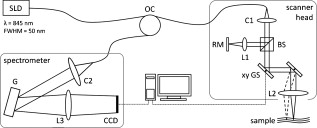
1.IntroductionFourier domain optical coherence tomography (FD OCT) is a special form1, 2 of OCT, which detects the spectral fringe signal of a full sample depth structure in the spatial domain by using a spectrometer-based system3, 4 (spectral domain OCT, SD OCT) or in time-domain by using a frequency-swept light source, optical frequency domain imaging5, 6 (OFDI). The detected depth-dependent modulation frequency of the light source spectrum is then analyzed by a Fourier transform, which provides the information on the amplitude and the phase of the light backscattered from within the sample.7 The axial velocity component of a moving scatterer causes a Doppler phase shift in the spectral interferometric signal. With this, absolute sample velocities can be determined by evaluating the phase differences between adjacent depth scans (A-scans) in a 2-D OCT image (B-scan). This functional extension of OCT is called phase-resolved Doppler OCT (DOCT) and promises clinical applications in imaging and characterization of in vivo blood flow, particularly in the human retina,8, 9, 10, 11, 12, 13 due to the high imaging speed and sensitivity14, 15 in SD OCT. This technique can be complicated due to motion artifacts resulting in phase instabilities and a low signal-to-noise ratio (SNR) caused by the motion induced interference fringe washout.9, 16 To avoid the effect of interference fringe blurring and the resulting signal power decrease due to sample motion, A. Bachmann proposed the resonant Doppler flow imaging,17 which generates a variable phase delay in the reference arm to enhance the backscattering signal of the moving sample. The quantitative flow velocity is determined by comparing the intensity signal with moving reference arm to the one with resting reference plane. The quantitative phase-resolved Doppler flow measurement in SD OCT acts on the assumption that the phase difference of sequential A-scans is linearly related to the flow velocity as where the parameter denotes the phase shift between consecutive A-scans, is the center wavelength of the OCT system, shows the refractive index, represents the time required for the detection of one A-scan, and is the Doppler angle between the direction of the moving object and the horizontal schematically drawn in Fig. 1 . Fig. 1Schematic showing the geometry of the incident sample beam relative to the 1% Intralipid solution flowing through the glass capillary. The angle represents the measured Doppler angle.  But this general assumption holds true only for almost purely axial motion. Lately, a new phase-dependent Doppler model was presented by our group,18, 19 which takes the transverse component of the oblique motion into account. This new Doppler model reveals that the effective axial displacement during the integration time is reduced and with this the phase shift is smaller than expected with the classic Doppler model. We also showed that for high axial velocity components, and with that large Doppler angles between the flow and the transverse direction, the classic Doppler model operates in good approximation with relative deviations smaller than 1%. In contrast to this, for small Doppler angles and high flow velocities, the phase shift between adjacent A-scans will approach a constant value making it impossible to quantify the flow velocity. For many in vivo blood flow measurements, especially 3-D flow imaging, random and unpredictable Doppler angles occur so that the undesirable small Doppler angles can not be precluded. Recent developments are focused on techniques for the qualitative imaging of blood perfusion in the human retina and choroid. For the decision weather or not a blood flow exists, the quantitative measurement of the phase shift and the flow velocity is not relevant. First, noninvasive optical retinal angiography was presented by S. Makita 20 using the phase-resolved Doppler analysis to contrast blood vessels. Another technique based on the phase information of the backscattered light is the optical angiography (OAG), which imposes a constant modulation frequency by moving the reference mirror during the A-scan acquisition to achieve the separation between moving and static structures.21, 22 An enhancement of OAG is the single-pass volumetric bidirectional blood flow imaging (SPFI) by Tao using a modified Hilbert transform algorithm to introduce a constant Doppler frequency shift without the necessity for a moving reference arm.23 Lately, the ultra-high-speed SD OCT, achieved by applying a novel CMOS detector, has shown its potential for 4-D Doppler imaging of human retinal blood flow.24 All of these techniques have presented impressive volumetric tomographies by using the example of the human retinal and choroidal vasculature. As indicated by Schmoll,24 not only the imaging of the vasculature is aspired to, but rather the quantification of blood flow, which offers the determination of physiological parameters and functional impairment of diseases. In this regard, quantitative 3-D in vivo measurements were presented using resonant Doppler OCT (Ref. 17), SPFI (Ref. 25), and the joint spectral and time domain OCT (STdOCT) (Ref. 26). Until now, however, the phase-resolved Doppler analysis with SD OCT is the most often used method for the quantitative flow measurement8, 9, 10, 11, 12, 13 because of the high phase stability. As a result of the new phase-resolved Doppler model, for small Doppler angles, which are conceivable particularly in the quantitative in vivo blood flow measurement, our proposal is to extend the limited velocity detection range of the Doppler method in SD OCT by taking the signal damping into account. In a previous study,27 we observed that the signal power decrease due to oblique sample motion is not just the sum of the axial and transverse effect16 but shows a specific characteristic depending on the Doppler angle set. This study implements this beneficial effect for quantitative flow velocity measurements. Therefore, we first recall the improved theoretical model for the Doppler phase shift and present—derived from this model—the numerically evaluated signal damping as a function of the oblique sample motion visualized in a universally valid contour plot. Both the limitation of the phase-resolved Doppler analysis at small Doppler angles as well as the feasibility of the signal power damping method to quantify flow velocities exceeding the reliable Doppler measurement range are evaluated using a flow phantom model with a 1% Intralipid emulsion. The quantitative combination of both methods is described based on standard deviations. Finally, a first in vivo measurement in the mouse model is presented where the arterial blood flow is quantified by the combination of Doppler and the signal damping method. 2.Theoretical Model2.1.Doppler Phase Shift and Mean SignalA detailed description of the theoretical models for the Doppler phase shift and the signal power decrease as functions of the absolute velocity of an obliquely moving sample can be found in Refs. 18, 19, 27. Therefore, the improved theory is mentioned briefly in this section. The oblique sample motion is described by an axial and transverse component during the integration time of the line detector of the SD OCT system. These parameters as well as the time are transformed into dimensionless coordinates as shown in Eqs. 2, 3, 4, where is the beam width (FWHM) of the Gaussian sample beam, is the center wavelength, and is the refractive index of the investigated sample. Based on the theory of Yun for a small spectral bandwidth of the SD OCT system,16 the photocurrent containing the interference modulation is integrated over with a result that is proportional to Eq. 5, where is the coordinate at , and is the complex amplitude of the light backscattered from the scatterer :For the Doppler analysis, the phase shift between subsequent A-scans of the time intervals and [0,1] is calculated by multiplying the complex amplitude of the first A-scan with the complex conjugate one of the consecutive A-scan. Because many different scatterers within the sample beam during contribute to the interference signal, the average is considered which corresponds to the argument of the mean value of [Eqs. 6, 7]:withandThe motion-induced signal power decrease can be described by the mean signal , which is the squared absolute value of the complex amplitude , as shown in Eq. 9. The damping of the signal is defined by the logarithmized mean signal .The integrals resulting from Eq. 6 for and Eq. 9 for can be solved analytically only for the case of purely axial motion.18, 19, 27 For finite transverse displacements of the sample motion, these integrals are numerically solved using Mathematica® 6.0 (Wolfram Research, Inc.). The resulting and values are presented each by a contour plot in Fig. 2 as functions of the normalized axial and transverse displacement in the range of 0 to 4. The results of in Fig. 2 were described in detail in previous studies.18, 19 In Fig. 2, the logarithmized is shown in steps of and color-separated in intervals of . The signal power decrease resulting from a purely axial motion is shown16, 27 by the vertical axis and follows In accordance with Ref. 16, in decibels can be described by for the purely transverse sample motion. The simulated values of and for a certain Doppler angle can be read from a linear slope through the origin of the coordinate system. The Doppler angle in the experimental setup is not identical to the angle in the contour plot. The transformation is presented byFig. 2(a) Contour plot of the average phase shift between sequential A-scans as a function of the normalized transverse (horizontal) and axial (vertical) displacement of the oblique sample motion and (b) the damping of the mean signal due to oblique sample motion is also shown by a universally valid contour plot. The presented lines with values of 39 and correspond to theoretical values compared with the experimental data presented in Sec. 4 [cf. Figs. 5, 6, 10, 10].  Fig. 5(a) Points: measured phase shifts in the interval of as a function of the calculated velocity assuming a parabolic flow profile. The Doppler angle is , resulting in of in the contour plots in Fig. 2. The velocity range of the 12 single measurements corresponds to from . Dashed line, calculated phase shift assuming a linear dependence of the phase shift from the axial velocity (classic Doppler model); solid line, as a function of in accordance to the new Doppler model by considering the measured beam width of . (b) Flow velocities (index , points with interpolated lines) determined by considering the new Doppler model as a function of the radial position compared to the theoretical prediction (index , solid line). Since the velocity can not be quantified unambiguously for and larger than , velocity profiles are presented for up to .  Fig. 6(a) Points: signal power decrease of the 1% Intralipid flow at from as a function of the absolute flow velocity at of . Solid line, theoretical prediction of the signal damping of the new model. As supposed by the simulation [Fig. 2], the signal power decreases monotonously with increasing flow velocity. (b) Flow profiles (index ) quantified by the signal damping and its theoretical prediction (index ) for ranging from . For the measurements with starting from , the Doppler SD OCT is no longer applicable [cf. Fig 5].  Fig. 10(a) Relationship of the phase shift in the interval of and the absolute sample velocity . The Doppler angle of corresponds to of in the contour plots in Fig. 2: solid line, result of the new Doppler model considering the spot size of ; dashed line, result of the classic Doppler model. (b) Corresponding damping of the mean signal as a function of the velocity for of .  Astonishingly, for the case of oblique sample motion, and do not follow the widely used classic Doppler model, which considers just the sum of the axial and transverse effect. As a result, for , the phase shift never reaches and oscillates at most around . With decreasing angles , approaches a constant value at higher velocities, making it difficult to quantify flow velocities on the basis of . The result of in Fig. 2 shows that points of total fringe washout at do not occur for any Doppler angle set. Instead of this, only oscillations in the signal power decrease appear if the axial displacement during is at least within the sample beam with the spot size . The explanation for this unexpected characteristic of the phase shift and the mean signal is based on the fact that the scattering particles are not present in the sample beam during the entire integration time leading to a reduced effective axial displacement . 2.2.Flow Measurement by Signal Power DecreaseConsidering the results of the numerical simulation, it becomes apparent that the Doppler flow measurement is limited in use for because reaches a value less than or equal to for higher velocities. Since this angle range can not be prevented, particularly in the quantitative in vivo blood flow measurement, we propose to extend the limited velocity detection range of the Doppler analysis in SD OCT by taking the monotone signal damping into account. For this kind of flow measurement, a few conditions must be fulfilled. First, the backscattering signal of the flowing medium with the homogenously distributed scattering particles must be higher than the noise level of the OCT system. Second, the signal-damping method requires a reference that contains the signal power at a defined velocity to calculate the signal decrease at a velocity indeterminable for Doppler SD OCT. For this, the often-measured arterial pulsatile blood flow offers a large velocity range between systole and diastole, where the latter is usable as a reference. The diastolic flow velocity is very slow, so that and are generally much smaller than 1 and with this are quantifiable using the Doppler analysis. The higher systolic blood flow velocity is then quantified by calculating the signal decrease relative to the diastolic point of time and assuming that the scattering properties of blood do not change between systole and diastole. The experimental flow measurement using the signal decay is presented first by a flow phantom model and second in the in vivo mouse model in Sec. 4. 3.Experimental Setup3.1.SD OCT SystemThe measurement system used in this study is based on fiber-coupled SD OCT with a free-space Michelson interferometer (see Fig. 3 ) and was previously described.27 The light source is a superluminescent diode (SLD 371 MP, Superlumdiodes Ltd., Russia) with a spectral bandwidth of (FWHM) and a center wavelength of . The light of the SLD is guided to the 3-D scanner head by an optical circulator (OC, Thorlabs, USA). The scanner head contains a collimator (C1) to generate a free-space beam, which is divided into a reference arm and a sample arm by a 20:80 beamsplitter (BS). The sample beam is deflected by two galvanometer scanners ( GS, Cambridge Technology Inc., USA) and focused on the sample with telecentric optics and a measured FWHM of the intensity profile of . The backscattered light is superimposed with the reference light and again coupled into the optical circulator. The self-designed spectrometer in the detection arm contains a collimator (C2), a reflective gold grating (G), and the lens system (L3) for focusing the interference fringes at a CCD line scan detector (DALSA IL C6, DALSA, USA). The integration time of the line detector amounts to which corresponds to an A-scan rate of at a duty cycle of 100%. The galvanometer scanners and the detector are triggered by an analog input/output card (National Instruments, USA). The acquisition and the processing of the experimental data are realized by means of a personal computer and custom software developed with LabVIEW (National Instruments, USA). 3.2.In Vitro Capillary ModelTo present the potential of the signal power decrease in the SD OCT for extending the limited Doppler velocity detection range at angles , a flow phantom model was used. In this experiment, a 1% Intralipid emulsion flowing through a glass capillary with an inner diameter of (Paul Marienfeld GmbH & Co. KG, Germany) was imaged two-dimensionally. The laminar flow of the turbid emulsion was ensured by an infusion pump (Fresenius Kabi AG, Germany) and a Reynolds number for all experiments. The flow rates were set from , corresponding to mean velocities of . The capillary was submerged in water to reduce optical distortion effects. The center of the capillary was positioned at the sample arm focus. Before imaging the flowing Intralipid, a volume scan was detected to measure the Doppler angle resulting in which corresponds to of in the contour plots in Fig. 2. For the flow quantification by Doppler SD OCT and SD OCT signal damping, time-resolved B-scans were acquired with a transverse displacement of the sample beam of . The resulting oversampling effect was revoked in the signal processing. 3.3.In Vivo Mouse ModelThe experiment in the in vivo mouse model represents a pilot study as part of a main research project considering the vasodynamics and its influence on the hemodynamics at the early stage of atherosclerosis.28 In this feasibility study, the combination of the phase-resolved Doppler SD OCT and the SD OCT signal power damping method were tested by experimental data of the saphenous artery of the right leg of a male C57BL/6 mouse under resting conditions without the use of vasoactive stimuli. Before examination, the mouse has been narcotized by intraperitoneal application of 95% ketamine combined with 5% xylazine using a dose of per of body weight. Because of the highly scattering properties of the fur covering the saphenous artery, the skin of the right hind leg was incised to gain access to the vessel. Therefore, only a connective tissue layer of about sits above the artery. To quantify the blood flow velocities, temporally resolved B-scans with a transverse displacement of the sample beam of were acquired. The Doppler angle of was measured from a 3-D data set and corresponds to of in the contour plots in Fig. 2. The procedure was approved by the Institutional Ethics Commission for Animal Experiments of the medical faculty of the University of Technology Dresden and the government of Saxony. 4.Results4.1.In Vitro Capillary ModelIn Fig. 4 , cross-sectional Doppler flow and structural SD OCT images of the flowing Intralipid through a glass capillary are presented for six different mean velocities ranging from and a set Doppler angle of . In the Doppler SD OCT images, the determined phase shifts are shown by a grayscale for the range of 0 to . Here, is calculated by multiplying the complex Fourier coefficient of one A-scan with the complex conjugate coefficient of the subsequent A-scan in each depth , where is the A-scan number.10, 12, 18, 29 The result, in turn, is a complex value with as the argument. For the averaging of of adjacent A-scans, the complex data is averaged and the mean value of is computed from the resulting argument. For one image, nine adjacent complex A-scans and 15 complex B-scans were averaged to eliminate the oversampling effect and to reduce the strong speckle noise. As seen in the image series at the top (Fig. 4), emanating from the capillary center the phase shift becomes larger with increasing from . For a of , exceeds . As predicted by the new Doppler model, for higher flow velocities does not reach and exceed and consequently does not wrap to the primary interval of as expected by considering the classic Doppler model. Instead, amounts to a value of about independent of the flow velocity. Another interesting effect is the phase shift at the backside of the capillary, which was also seen in a previous study.30 In contrast, the front side of the capillary does not show this shift. Currently, this feature can only be explained by the assumption that light scattered forward from fast moving scatterers is reflected at the capillary backside, resulting in a phase shift different from zero and must be investigated in a future research. Fig. 4Cross-sectional Doppler flow (top) and structural SD OCT images (bottom) of the Intralipid flow through a glass capillary immersed in water at a Doppler angle of and six different mean velocities from . The phase shift is presented in the range from 0 to . The gray logarithmic amplitude scale represents a range of . The scale bar at the top of the images on the left shows a distance of . 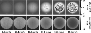 For the structural SD OCT images presented as series at the bottom of Fig. 4, the real parts of the complex Fourier coefficients of nine adjacent A-scans are averaged. Subsequently, 15 of the resulting real-valued B-scans were also averaged. The signal power presented in the logarithmic scale is ranging up to . It becomes apparent that a monotonously decreasing signal power occurs with increasing mean flow velocity up to the highest flow velocity measured. For the analysis of the cross section through the capillary center, 64 instead of only 15 B-scans were averaged in the manner already described to average a total of 576 single values for the mean values of and . Figure 5 shows the phase shifts of 12 measurements with mean velocities ranging from as a function of the calculated sample velocity assuming a parabolic flow profile. As seen, the data spans a velocity range up to approximately which corresponds to maximum displacements of 2.1 and of 1.7. The prediction of the classic Doppler model calculated by Eq. 1 is presented by the dashed line, showing large deviations at higher flow velocities. In addition, calculated from the new model is plotted as a black solid line and corresponds to the values of the linear slope at drawn in Fig. 2. We can see that the measured data correspond very well to the phase shift of the new Doppler model. Despite of an identical averaging used for the entire velocity range, the data at higher velocities show more noise, most likely caused by the random phases of particles present in the sample beam at only one of the considered A-scans for the Doppler calculation. Figure 5 presents the flow velocity profiles (index ) calculated by using the to relationship of the new Doppler model for [solid line in Fig. 5] as a function of the radial position of the capillary center in comparison to the theoretical prediction (index ) of the flow velocity according to the Hagen-Poiseuilles law. Here, the positive values of represent the backside of the capillary. As shown in Fig. 5, the flow velocity according to the new Doppler model can only be calculated unambiguously up to corresponding to a phase shift of . Unfortunately, higher flow velocities can not be determined by using for the presented experiment. As shown in the preceding section, a quantitative flow measurement by using the Doppler analysis is limited in use for at high flow velocities. Therefore, the signal damping as a function of the absolute sample velocity for the 12 measurements with ranging from is determined in the next step. As a reference, the signal power measured at zero flow is chosen. Figure 6 plots the logarithmized mean signal of the averaged A-scan at the capillary center against the calculated velocity , assuming a parabolic flow as well. As for the Doppler analysis, each of the shown data points relates to a mean value of 576 single measurements. The solid curve corresponds to the simulated values of the line with in Fig. 2. Despite the speckle noise, the measured data agree very well with the theory of the new model. Because the signal power decreases monotonously, the flow velocity can be calculated unambiguously. Figure 6 presents the resulting flow profiles (index ) in comparison to the theoretical profiles (index ). As seen, the measured values are in good agreement with the theory. At the border area of the capillary lumen, small deviations can be noticed, which are caused by the strong speckle noise relative to the minor signal damping at small flow velocities. By considering the experimental results, the question at which flow velocity the signal damping is preferred to the Doppler analysis is addressed in the following section. A weighted mean value of the velocities calculated by using the Doppler and the signal damping method can be determined by taking the error of both methods into account. For this, the weights of the velocity calculated by the Doppler phase shift and of the velocity determined by the signal damping are ascertained as presented in Eqs. 11, 12 where and are the standard deviations of and , respectively. As shown in Eq. 11, is calculated by the multiplication of the measured standard deviation of the phase shift with the derivation based on the inverted simulated curve [see the solid line in Fig. 5]. The standard deviation was presented by Park for the case of the discontinuous, purely transverse sample beam movement with the result that as function of can be described31 by a linear slope up to of 1.0. In the presented experiment, a standard deviation of was determined for the linear range. For the calculation of the value , as shown in Eq. 12, the standard deviation of the logarithmized mean signal was measured for the entire measurement range up to and results in a constant of due to the Rayleigh distribution of the OCT signal.32 The comparison of the weights normalized to its sum is presented in Fig. 7 . As seen, the weight of the velocity calculated by is decreasing with increasing velocity and approaches zero at the uniqueness limit of . On the contrary, the weight of the velocity determined by the signal power decrease is almost 0 for small velocities because of the strong speckle noise relative to the minor signal damping and is increasing for higher flow velocities. Consequently, flow velocities up to the intersection point of are dominated by the Doppler SD OCT for the presented experiment with . Higher flow velocities are quantified more precisely by the signal damping method. Figure 7 presents the weighted mean velocities of both methods calculated by Eq. 13 for eight representative measurements with of .As a result, the velocity measurement by using the signal damping in combination with the Doppler analysis is not only an alternative method but also provides the feasibility to extend the limited Doppler flow measurement range.Fig. 7(a) Normalized weight of the velocity determined by the Doppler analysis ( , dashed line) and of the velocity computed by using the signal damping method ( , solid line) as a function of the absolute flow velocity ranging from zero to the Doppler uniqueness limit of for . The intersection point at represents the point from which the flow velocity is more precisely calculated by the signal damping method. The range, in which the combined method can be used, extends the shown velocity range. (b) Weighted mean value of the flow velocities of both methods, the Doppler analysis and the signal damping, are calculated by taking the errors of and into account.  4.2.In Vivo Mouse ModelIn this experiment, data were acquired from the murine saphenous artery in vivo. The resulting grayscale cross-sectional Doppler flow and structural SD OCT images of three consecutive B-scans describing one cardiac cycle are presented in Fig. 8 . The measurement in Fig. 8 shows the systole, that in Fig. 8 relates to the point of time between systole and diastole, and that in Fig. 8 corresponds to the diastole. For one image, 10 adjacent A-scans were averaged in the way described in Sec. 4.1. In contrast to the experiments with the capillary model, a significant signal power attenuation of the flowing blood with increasing depth can be observed and is caused by the highly scattering properties of the blood for the wavelength range used.33 On closer examination of the Doppler flow images at the top of Fig. 8, we can notice that the phase shift shows a strong noise even at a sufficiently high signal power and despite of averaging 10 single values. The reason for this effect may be multiple scattering events causing a significant signal in larger depth and probably a noisy phase shift.34 Accordingly, the phase shift can be determined reliably only near the upper side of the vessel lumen. The damping of the mean signal is caused by the continuous phase change during the integration time and is consequentially related to the phase shift . From this it follows that the analyzable depth range for the signal damping is limited to the upper vessel part as well. To determine the feasibility of the blood flow measurement by the signal damping in combination with the Doppler method for SD OCT, the following analysis refers to the limited depth range of the vessel lumen. Fig. 8Gray-scale Doppler flow (top) and structural SD OCT images (bottom) of three consecutive B-scans of the saphenous artery in vivo under resting conditions. The scale bar represents a distance of . (a) Relates to the systole, (b) shows the point of time between systole and diastole and corresponds to the intermediate, and (c) represents the diastole.  Figure 9 shows the phase shift of the A-scan at the vessel center in the interval as a function of the radial position inside the artery for the intermediate (white diamonds) and the diastolic point of time (black diamonds). Here, the negative values of relate to the upper side of the vessel. Because at the systole only at the upper vessel part show reliable values of the phase shift, this measurement can be used neither for the Doppler analysis nor for the signal damping method. For the intermediate and the diastole, only the phase shifts for ranging from corresponding to 11 depth pixels are reliable and are used for fitting a parabolic profile. By means of this range, we can notice that the flow velocity is decreased from the intermediate to the diastole as expected. Figure 9 shows the corresponding signal power and the fit of a polynomial of second degree to the reliable measurement points against the parameter . Even for this small analyzable depth range, a signal power damping can be observed for the intermediate in comparison to the smaller diastolic blood flow. Fig. 9(a) Phase shift of the A-scan at the vessel center for the intermediate (white diamonds) and the diastole (black diamonds) as a function of the radial position . The diameter of the artery was determined by assuming a refractive index of blood of 1.4 and amounts to . The reliable values of can be found in the range . (b) Related signal power for the intermediate and the diastole and the fitted polynomials for the calculation of the absolute signal power damping of the intermediate.  For the measured reliable phase shifts of the intermediate and the diastolic point of time [cf. Fig. 9], the flow velocity values were determined by taking the result of the new Doppler model into account. The used relationship of the phase shift and the sample velocity for is presented by the solid line in Fig. 10 . In comparison, the result of the classic model is shown by the dashed line. The parabolic fit to the flow velocity of the diastole results in a maximum velocity of at the vessel center and an exponent of : The fitted flow velocity profile and the fitted signal power in the diastole provide the information for the calculation of the signal power decrease of the intermediate flow. By means of this signal damping and the result of the new model, the absolute flow velocity of the intermediate is then determined for . In Fig. 10, the utilized damping of the mean signal calculated by the new model corresponds to the solid line. Also, the degradation of by considering just the sum of the axial and transverse effect is presented by the dashed line, showing large deviations at higher flow velocities.Figure 11 presents the resulting blood flow velocities as a function of the radial position . There, the flow velocities of the intermediate and the diastole calculated by the new Doppler model (index ) are shown by the white and black diamonds, respectively. The fitted parabolic profile of the diastole with and corresponds to the thin solid line. The blood flow velocities of the intermediate point of time determined by the signal damping (index sd) are shown by the gray points, which are in excellent agreement with the reliable values determined with the Doppler analysis. The fit of the intermediate flow velocities results in and for both the Doppler and signal damping analyzed values. Fig. 11Detailed view of the flow velocity against the radial position in the range of : index flow velocities of the intermediate (white diamonds) and the diastole (black diamonds) calculated by considering the new Doppler model; index sd, the result of the velocity quantification of the intermediate flow by using the signal damping with the Doppler analyzed diastolic flow as a reference.  5.DiscussionThe experiments showed that the signal power decrease in combination with the Doppler analysis can be used for the flow measurement. For the routine use of this combined procedure in the in vivo mouse model as part of the vasodynamics research, an SD OCT system with a center wavelength of about should be used because of the reduced scattering and absorption of blood cells in this wavelength range. With this, it should be possible to extend the limited Doppler measurement range in SD OCT for by analyzing the signal damping at higher blood flow velocities. Additionally, note that the vessels being investigated must be close to the surface of the surrounding scattering tissue, so that a significant backscattering signal occurs. The influence of multiple scattering on the Doppler velocity profile was analyzed experimentally by Moger 34 This study has shown that the parabolic flow profile of the flowing whole human blood through a glass capillary becomes increasingly distorted at greater depths of the tissue phantom, consisting of a solution of 20% Intralipid, which may be due to the occurrence of multiple scattering events that cause both falsely registered depths and Doppler shifts. The result presented for tissue phantom above the glass capillary contains an only slightly changed parabolic profile. In contrast to larger depth relative to the tissue surface, one would expect a flattened and slightly broadened profile. These results were confirmed by Bykov 35 using a Monte-Carlo method for the simulation of the effect of position depth of a particle suspension flow in a light scattering medium on Doppler velocity profiles. Because the signal damping is related to the Doppler phase shift, the measured damping of the mean signal and consequently the resulting flow velocities are not credible as well for the case of multiple scattering. In the presented in vivo experiment, the structure above the saphenous artery is about , comparable to layer structures above retinal vessels8, 11, 22 and should cause only a slightly changed parabolic profile which correlates with the fitted exponent [see Eq. 14] for the diastolic and intermediate flow. Advantageously, the proposed signal damping method can also be used for flow measurement of moving particle solutions normal to the direction of the incident sample beam. For this purely transverse motion, a signal decrease occurs due to the numerous but smaller signals of arbitrary phase during compared to the smaller number of scatterers of a stationary sample [see the horizontal axis in the contour plot in Fig. 2]. Therefore, this method joins developments for overcoming the problem of oblique geometry such as speckle flow imaging.36 A drawback of the speckle flow imaging and the signal damping method is the missing information about the flow direction being available in Doppler measurements. The development37 of dual-beam Doppler SD OCT offers the possibility of absolute blood flow measurement regardless of the vessel orientation by using two sample beams with different Doppler angles. In this approach, two interferometers with a fixed optical path length difference, in both sample and reference arm, were used to avoid crosstalk. As for the Doppler SD OCT with only one sample beam, a limitation is given for blood flow with abrupt changing direction. Probably, systems based on dual-beam Doppler SD OCT (Refs. 37, 38) do not suffer from the washout of the interference fringes at physiological blood flow velocities, but complications resulting from considering just the classic relationship are not excluded. For example, for small Doppler angles corresponding to nearly transverse sample motion and high flow velocities in one sample beam, the phase shift will approach a constant value as well. If the angle between the two beams is about as presented in Ref. 37, the absolute Doppler angle considering the second sample beam would be around , resulting in a strong signal washout at higher flow velocities. Consequently, for this particular example, the determination of the absolute sample velocity turns out to be difficult despite of the double phase information. Accordingly, the combination of Doppler and signal damping method could also be a promising extension for flow measurements with dual-beam systems. 6.Summary and ConclusionRecently, we presented a new phase-resolved Doppler model for SD OCT that does not ignore the transverse component of oblique sample motion. In addition to the nonlinearity of the measured phase shift to the axial velocity component, it was shown that for small Doppler angles and high sample velocities, the phase shift will converge to a constant value. By using the prevalent classic Doppler model for the case of small Doppler angles and high flow velocities, the flow profiles computed are completely false, which can possibly lead to failing medical and clinical interpretations. Since in many Doppler applications small Doppler angles are unavoidable, we propose to determine the flow velocities accurately with the combination of the new Doppler model and the characteristic signal power decrease due to fringe washout in SD OCT. In this paper, the new relation of the signal damping and the oblique sample displacement was presented by a universal contour plot as a result of the numerical simulation. As for the Doppler phase shift, this diagram is valid for any SD OCT system with a particular center wavelength and the beam size . For the experimental verification, the limited velocity measurement range of the Doppler SD OCT was presented by using a capillary flow phantom model with a 1% Intralipid emulsion. The feasibility of the characteristic signal power decrease at a certain Doppler angle to quantify absolute flow velocities was presented by the same in vitro experiment and higher flow velocities. Furthermore, a weighting was calculated by considering the standard deviation of the Doppler phase shift and the signal power damping as functions of the sample velocity to determine which method is favored at a certain flow velocity and to calculate the weighted mean value of the velocities of both methods. The second analysis was performed at the acquired data set of the murine saphenous artery in vivo. The limitation of this in vivo measurement was not the Doppler analysis but the strong signal power decrease with increasing depth probably caused by the refractive index-mismatch of blood.33 Consequently, only the reliable range of the vessel lumen was analyzed concerning the Doppler phase shift and the signal power decrease. Accordingly, for future studies it is indispensable to use a SD OCT system with a center wavelength of about to image the entire depth range of the saphenous artery. In this context, it is also necessary to investigate the influence of the pulsatile blood flow on the distribution of the blood cells within the vessel. A first indication was given in a previous study39 showing that the erythrocytes are not present in the vessel center and close to the vessel wall. For the blood flow measurement using the combination of Doppler analysis and signal damping method, it is essential that the distribution of the scatterers is not changed with respect to the reference measurement. In conclusion, we presented that a quantitative flow measurement by means of the characteristic signal damping shows great promise to extend the limited velocity measurement range of the Doppler SD OCT analysis at small Doppler angles and high flow velocities. In a prospective study, we would like to evaluate this technique for the in vivo blood flow measurement by using a SD OCT system. AcknowledgmentsThis research was supported by SAB (Saechsische Aufbaubank, project: 11261/1759), the BMBF (Bundesministerium für Bildung und Forschung: NBL 3), and the MeDDrive program of the Medical Faculty Carl Gustav Carus of the Dresden University of Technology. ReferencesD. Huang, E. A. Swanson, C. P. Lin, J. S. Schuman, W. G. Stinson, W. Chang, M. R. Hee, T. Flotte, K. Gregory, C. A. Puliafito, and J. G. Fujimoto,
“Optical coherence tomography,”
Science, 254
(5035), 1178
–1181
(1991). https://doi.org/10.1126/science.1957169 0036-8075 Google Scholar
A. F. Fercher, W. Drexler, C. K. Hitzenberger, and T. Lasser,
“Optical coherence tomography—principles and applications,”
Rep. Prog. Phys., 66
(2), 239
–303
(2003). https://doi.org/10.1088/0034-4885/66/2/204 0034-4885 Google Scholar
A. F. Fercher, C. K. Hitzenberger, G. Kamp, and S. Y. El Zaiat,
“Measurement of intraocular distances by backscattering spectral interferometry,”
Opt. Commun., 117
(1–2), 43
–48
(1995). https://doi.org/10.1016/0030-4018(95)00119-S 0030-4018 Google Scholar
G. Häusler and M. W. Lindner,
“‘Coherence radar’ and ‘Spectral radar’—new tools for dermatological diagnosis,”
J. Biomed. Opt., 3
(1), 21
–31
(1998). https://doi.org/10.1117/1.429899 1083-3668 Google Scholar
S. R. Chinn, E. A. Swanson, and J. G. Fujimoto,
“Optical coherence tomography using a frequency-tunable optical source,”
Opt. Lett., 22 340
–342
(1997). https://doi.org/10.1364/OL.22.000340 0146-9592 Google Scholar
U. H. P. Haberland, V. Blazek, and H. J. Schmitt,
“Chirp optical coherence tomography of layered scattering media,”
J. Biomed. Opt., 3 259
–266
(1998). https://doi.org/10.1117/1.429889 1083-3668 Google Scholar
R. Leitgeb, M. Wojtkowski, A. Kowalczyk, C. K. Hitzenberger, M. Sticker, and A. F. Fercher,
“Spectral measurement of absorption by spectroscopic frequency-domain optical coherence tomography,”
Opt. Lett., 25 820
–822
(2000). https://doi.org/10.1364/OL.25.000820 0146-9592 Google Scholar
R. A. Leitgeb, L. Schmetterer, W. Drexler, A. F. Fercher, R. J. Zawadzki, and T. Bajraszewski,
“Real-time assessment of retinal blood flow with ultrafast acquisition by color Doppler Fourier domain optical coherence tomography,”
Opt. Express, 11 3116
–3121
(2003). https://doi.org/10.1364/OE.11.003116 1094-4087 Google Scholar
B. R. White, M. C. Pierce, N. Nassif, B. Cense, B. H. Park, G. J. Tearney, B. E. Bouma, T. C. Chen, and J. F. de Boer,
“In vivo dynamic human retinal blood flow imaging using ultra-high-speed spectral domain optical Doppler tomography,”
Opt. Express, 11 3490
–3497
(2003). https://doi.org/10.1364/OE.11.003490 1094-4087 Google Scholar
H. Wehbe, M. Ruggeri, S. Jiao, G. Gregori, C. A. Puliafito, and W. Zhao,
“Automatic retinal blood flow calculation using spectral domain optical coherence tomography,”
Opt. Express, 15 15193
–15206
(2007). https://doi.org/10.1364/OE.15.015193 1094-4087 Google Scholar
Y. Wang, B. A. Bower, J. A. Izatt, O. Tan, and D. Huang,
“In vivo total retinal blood flow measurement by Fourier domain Doppler optical coherence tomography,”
J. Biomed. Opt., 12 041215
(2007). https://doi.org/10.1117/1.2772871 1083-3668 Google Scholar
B. A. Bower, M. Zhao, R. J. Zawadzki, and J. A. Izatt,
“Real-time spectral domain Doppler optical coherence tomography and investigation of human retinal vessel autoregulation,”
J. Biomed. Opt., 12 041214
(2007). https://doi.org/10.1117/1.2772877 1083-3668 Google Scholar
Y. Wang, A. Fawzi, O. Tan, J. Gil-Flamer, and D. Huang,
“Retinal blood flow detection in diabetic patients by Doppler Fourier domain optical coherence tomography,”
Opt. Express, 17 4061
–4073
(2009). https://doi.org/10.1364/OE.17.004061 1094-4087 Google Scholar
R. Leitgeb, C. K. Hitzenberger, and A. F. Fercher,
“Performance of fourier domain vs. time domain optical coherence tomography,”
Opt. Express, 11 889
–894
(2003). https://doi.org/10.1364/OE.11.000889 1094-4087 Google Scholar
M. A. Choma, M. V. Sarunic, C. Yang, and J. A. Izatt,
“Sensitivity advantage of swept source and Fourier domain optical coherence tomography,”
Opt. Express, 11 2183
–2189
(2003). https://doi.org/10.1364/OE.11.002183 1094-4087 Google Scholar
S. H. Yun, G. J. Tearney, J. F. de Boer, and B. E. Bouma,
“Motion artifacts in optical coherence tomography with frequency-domain ranging,”
Opt. Express, 12 2977
–2998
(2004). https://doi.org/10.1364/OPEX.12.002977 1094-4087 Google Scholar
A. H. Bachmann, M. L. Villiger, C. Blatter, T. Lasser, and R. A. Leitgeb,
“Resonant Doppler flow imaging and optical vivisection of retinal blood vessels,”
Opt. Express, 15 408
–422
(2007). https://doi.org/10.1364/OE.15.000408 1094-4087 Google Scholar
E. Koch, J. Walther, and M. Cuevas,
“Limits of Fourier domain Doppler-OCT at high velocities,”
Sens. Actuators, A, 156
(1), 8
–13
(2009). https://doi.org/10.1016/j.sna.2009.01.022 0924-4247 Google Scholar
J. Walther and E. Koch,
“Transverse motion as a source of noise and reduced correlation of the Doppler phase shift in spectral domain OCT,”
Opt. Express, 17 19698
–19713
(2009). https://doi.org/10.1364/OE.17.019698 1094-4087 Google Scholar
S. Makita, Y. Hong, M. Yamanari, T. Yatagai, and Y. Yasuno,
“Optical coherence angiography,”
Opt. Express, 14 7821
–7840
(2006). https://doi.org/10.1364/OE.14.007821 1094-4087 Google Scholar
R. K. Wang, S. L. Jacques, Z. Ma, S. Hurst, S. R. Hanson, and A. Gruber,
“Three dimensional optical angiography,”
Opt. Express, 15 4083
–4097
(2007). https://doi.org/10.1364/OE.15.004083 1094-4087 Google Scholar
L. An and R. K. Wang,
“In vivo volumetric imaging of vascular perfusion within human retina and choroids with optical micro-angiography,”
Opt. Express, 16 11438
–11452
(2008). https://doi.org/10.1364/OE.16.011438 1094-4087 Google Scholar
Y. K. Tao, A. M. Davis, and J. A. Izatt,
“Single-pass volumetric bidirectional blood flow imaging spectral domain optical coherence tomography using a modified Hilbert transform,”
Opt. Express, 16 12350
–12361
(2008). https://doi.org/10.1364/OE.16.012350 1094-4087 Google Scholar
T. Schmoll, C. Kolbitsch, and R. A. Leitgeb,
“Ultra-high-speed volumetric tomography of human retinal blood flow,”
Opt. Express, 17 4166
–4176
(2009). https://doi.org/10.1364/OE.17.004166 1094-4087 Google Scholar
Y. K. Tao, K. M. Kennedy, and J. A. Izatt,
“Velocity-resolved 3D retinal microvessel imaging using single-pass flow imaging spectral domain optical coherence tomography,”
Opt. Express, 17 4177
–4188
(2009). https://doi.org/10.1364/OE.17.004177 1094-4087 Google Scholar
A. Szkulmowska, M. Szkulmowski, D. Szlag, A. Kowalczyk, and M. Wojtkowski,
“Three-dimensional quantitative imaging of retinal and choroidal blood flow velocity using joint spectral and time domain optical coherence tomography,”
Opt. Express, 17 10584
–10598
(2009). https://doi.org/10.1364/OE.17.010584 1094-4087 Google Scholar
J. Walther, A. Krueger, M. Cuevas, and E. Koch,
“Effects of axial, transverse and oblique motion in FD OCT in systems with global or rolling shutter line detector,”
J. Opt. Soc. Am. A, 25 2791
–2802
(2008). https://doi.org/10.1364/JOSAA.25.002791 0740-3232 Google Scholar
S. Meissner, G. Mueller, J. Walther, H. Morawietz, and E. Koch,
“In-vivo Fourier domain optical coherence tomography as a new tool for investigation of vasodynamics in the mouse model,”
J. Biomed. Opt., 14 034027
(2009). https://doi.org/10.1117/1.3149865 1083-3668 Google Scholar
L. Wang, Y. Wang, S. Guo, J. Zhang, M. Bachman, G. P. Li, and Z. P. Chen,
“Frequency domain phase-resolved optical Doppler and Doppler variance tomography,”
Opt. Commun., 242 345
–350
(2004). https://doi.org/10.1016/j.optcom.2004.08.035 0030-4018 Google Scholar
R. A. Leitgeb, L. Schmetterer, C. K. Hitzenberger, A. F. Fercher, F. Berisha, M. Wojtkowski, and T. Bajraszewski,
“Real-time measurement of in vitro flow by Fourier-domain color Doppler optical coherence tomography,”
Opt. Lett., 29 171
–173
(2004). https://doi.org/10.1364/OL.29.000171 0146-9592 Google Scholar
B. H. Park, M. C. Pierce, B. Cense, S. H. Yun, M. Mujat, G. J. Tearney, B. E. Bouma, and J. F. de Boer,
“Real-time fiber-based multi-functional spectral-domain optical coherence tomography at ,”
Opt. Express, 13 3931
–3944
(2005). https://doi.org/10.1364/OPEX.13.003931 1094-4087 Google Scholar
B. Karamata, K. Hassler, M. Laubscher, and T. Lasser,
“Speckle statistics in optical coherence tomography,”
J. Opt. Soc. Am. A, 22 593
–596
(2005). https://doi.org/10.1364/JOSAA.22.000593 0740-3232 Google Scholar
M. Brezinski, K. Saunders, C. Jesser, X. Li, and J. Fujimoto,
“Index matching to improve optical coherence tomography imaging through blood,”
Circulation, 103 1999
–2003
(2001). 0009-7322 Google Scholar
J. Moger, S. J. Matcher, C. P. Winlove, and A. Shore,
“The effect of multiple scattering on velocity profiles measured using Doppler OCT,”
J. Phys. D Appl. Phys., 38 2597
–2605
(2005). https://doi.org/10.1088/0022-3727/38/15/010 Google Scholar
A. V. Bykov, M. Y. Kirillin, and A. V. Priezzhev,
“Analysis of distortions in the velocity profiles of suspension flows inside a light-scattering medium upon their reconstruction from the optical coherence Doppler tomograph signal,”
Quantum Electron., 35 1079
–1082
(2005). https://doi.org/10.1070/QE2005v035n11ABEH012792 1063-7818 Google Scholar
J. Barton and S. Stromski,
“Flow measurement without phase information in optical coherence tomography images,”
Opt. Express, 13 5234
–5239
(2005). https://doi.org/10.1364/OPEX.13.005234 1094-4087 Google Scholar
N. V. Iftimia, D. X. Hammer, R. D. Ferguson, M. Mujat, D. Vu, and A. A. Ferrante,
“Dual-beam Fourier domain optical Doppler tomography of zebrafish,”
Opt. Express, 16 13624
–13636
(2008). https://doi.org/10.1364/OE.16.013624 1094-4087 Google Scholar
R. M. Werkmeister, N. Dragostinoff, M. Pircher, E. Götzinger, C. K. Hitzenberger, R. A. Leitgeb, and L. Schmetterer,
“Bidirectional Doppler Fourier-domain optical coherence tomography for measurement of absolute flow velocities in human retinal vessels,”
Opt. Lett., 33 2967
–2969
(2008). https://doi.org/10.1364/OL.33.002967 0146-9592 Google Scholar
J. Moger, S. J. Matcher, C. P. Winlove, and A. Shore,
“Measuring red blood cell flow dynamics in a glass capillary using Doppler optical coherence tomography and Doppler amplitude optical coherence tomography,”
J. Biomed. Opt., 9 982
–994
(2004). https://doi.org/10.1117/1.1781163 1083-3668 Google Scholar
|