|
|
1.IntroductionCurrently, retinal diseases are only treated after pathological changes and loss of vision have already occurred. It is believed that probing retinal physiology in vivo, in a noninvasive way could, in the future, provide a method to detect ophthalmological diseases at a very early stage, even before pathological changes are detectable with the current diagnostic tools. Furthermore, the unique possibility to study the physiology of neural retinal tissue in a complete noninvasive and noncontact way raised the interest of several research groups. In vitro studies of the phototransduction process in animal retina lead to detailed biochemical models.1 However, due to the limited physical access to the retina, the availability of techniques allowing assessing human retinal signal pathways and photoreceptor functionality in vivo are limited. Optical detection methods, on the other hand, profit from natural access to retinal structure. They have been proven successful to detect retinal reflectivity changes as response to light stimuli and thus indicate a direction for probing of retinal functionality in a completely noninvasive way.2, 3, 4, 5 Currently used methods can be roughly categorized into fundus imaging methods and optical coherence tomography (OCT) techniques. Full field techniques equipped with fast camera technology or scanning laser ophthalmoscopes (SLO) have the advantage of comprehensive motion artifact-free imaging for single frames.6, 7 The disadvantage of fast 2-D imaging techniques is the reduced depth sectioning capability. This is provided by OCT, where depth localization is given by the temporal coherence properties of the probing light.8 Early experiments in the field of optical assessment of retinal physiology provided evidence of flicker-evoked changes in retinal blood flow and extracellular pH in animals.9, 10, 11 The first application of time-domain OCT (TDOCT) to intrinsic retinal imaging was demonstrated on excised but alive small animal retina.12 Reflectivity changes in the outer photoreceptor segment have been observed. Fourier-domain OCT (FDOCT) has largely replaced TDOCT due to its higher speed and sensitivity.13 Recently presented ultrahigh-speed FDOCT systems allow recording depth resolved retinal sections in vivo at an acquisition speed of multiple volumes per second, while maintaining good image quality.14, 15 Testing the functionality of rat retina demonstrated the imaging capabilities of FDOCT to perform intrinsic imaging in the living animal.16 Once again a significant change of reflectivity within the photoreceptor outer segment has been reported. In vivo studies of reflectivity changes on human retina are challenging due to various sources of error, such as eye motion and the presence of speckle. Srinivasan recently presented results of intrinsic scattering changes in the human retina using FDOCT.17 In their experiment, they recorded a volume series at an acquisition speed of six volumes/s during , revealing a response occurring in the first after onset of a continuous light stimulus. An impressive example for imaging and probing retinal function with flash stimuli in humans on the level of individual cone photoreceptors using an adaptive optics (AO) flood illumination camera was presented by Jonnal 7 With the high frame rate of of a flood illumination camera, they were able to discover fast responses in the photoreceptors, lasting only . Applying AO SLO, Grieve and Roorda6 successfully imaged changes in reflectivity of human retina as response to a flicker stimulus at . In contrast to Jonnal 7 they found changes, which rose for the duration of the flicker over several seconds and dropped quickly back to baseline right after stimulus offset. Single-point measurements with FDOCT using a light source centered in the near-infrared region at have been demonstrated by the group of Drexler.18 This wavelength range has the advantage of allowing efficient decoupling of excitation and probing spectra. Thus far, the drawbacks of spectrometer-based FDOCT at are limited availability and the cost of high-speed array detector technology operating in the infrared region. It is clearly challenging to record signal changes in vivo of only a few percent. As outlined by many authors, the most problematic sources of noise is eye motion during stimulus response recording. Also, heartbeat or blood flow might introduce critical intensity fluctuations of backscattered light. The aim of the current work is therefore to introduce a new experimental approach that effectively reduces the influence of low-frequency–noise (1/f-noise) components and enhances sensitivity by making use of a heterodyne detection concept. We apply a localized stimulus flickering at the retina at a defined frequency. The assumption is that the backscattered intensity from responsive retinal tissue follows the periodic stimulus at exactly the same frequency. Hence, filtering the measured FDOCT signal at such heterodyne frequency will have the desired effect of suppressing previously described unwanted 1/f-noise contributions. An important parameter for this approach is the flicker frequency for which an optimum response can be measured. Furthermore, the temporal shape of the response signal might not necessarily be a sinusoidal function. Finally, it is important to understand the influence of FDOCT probing spot size to the amount of signal fluctuations. Those parameters are addressed in prestudies presented in the technical part of this paper. 2.Methods2.1.Optical SetupFigure 1 shows the optical setup. We use a superluminescence diode [(SLD), spectral width centered at , EXALOS Inc.] providing a theoretical axial resolution in air of . The light of the sample arm is scanned via an galvanometer-scanner unit, and directed to the eye through a telescope (L1-L2). For the measurements presented in this paper, we used two telescope settings: , for imaging with a large spot size on the retina (Table 1 , setting B and C), , and for high transverse resolution imaging (Table 1, setting A). For the high transverse resolution setting, we additionally introduced a telescope (L3-L4) in the sample arm, in order to further enlarge the beam diameter. The corresponding beam diameters at the cornea were and , with theoretical diffraction limited spot sizes on the retina of 62.3 and , respectively. Dispersion is compensated by a prism pair and a water chamber in the reference arm. The reference mirror is mounted on a translation stage. At the exit of the interferometer, the light from sample and reference path is guided through a single-mode fiber to the spectrometer. The latter consists of a transmission diffraction grating (Wasatch, ), an achromatic camera lens , and a high-speed CMOS line sensor (BASLER Sprint spL4096- , , ). Fig. 1Experimental setup. (a) Optical setup: SLD, superluminesence diode; PC, polarization controller; FC, fiber coupler; BS, beamsplitter; DISP, dispersion compensation; M, mirror; L, lens; SC, scanner; D, dichroic mirror; P, stimulus pattern; DG, diffraction grating; LSC, line scan camera. (b) Fundus projection: Yellow squares indicate the stimulus position; red dot indicates the probing position of the single spot experiments; and red line indicates the probing position of the B-scan time series. (c) Stimulus and probing spectra. (Color online only.)  Table 1Experiment parameters.
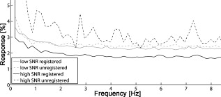
The effective maximum speed of the detector is defined by the number of horizontal pixels, chosen for read out. For the presented experiments, we used allowing for a maximum line rate of . We image the spectral half width of the SLD of onto of the sensor resulting in a full depth range in air of . In order to support the theoretical axial resolution, we increase the axial sampling by twofold zero padding before applying the Fourier transform.19 For the optophysiology experiments (Table 1, setting B and C), the power incident at the cornea was intentionally set to as discussed in Section 2.2. For the ultrahigh-speed measurements (Table 1, setting A), we used a power incident at the cornea , which is still safe for direct beam viewing according to laser safety standards. For introducing flash stimuli, we built a frequency- and color-controllable RGB unit, which consists of three high-power LEDs at red , green , and blue [Fig. 1]. They illuminate a mask, which is imaged via the telescope (L1-L2) onto the retina [see Fig. 1]. The mask contains two square areas for stimulation as well as a small spot in the middle to ease eye fixation for the volunteer. For the stimulus, we use an additive mixture of red and green [Fig. 1]. The stimulus position was chosen within the illuminated square superior and inferior to the fovea at an eccentricity of [see Fig. 1]. The volunteer’s pupil has been dilated for all experiments including flicker stimulation, using tropicamide. The total stimulus power amounted to , which again is safe according to laser safety standards. We dark-adapted the volunteer for prior to the experiments. 2.2.Measurement ParametersThe measurement parameters for assessing neural retinal responses in humans in vivo needs particular attention since one operates in a highly multidimensional parameter space. Figure 2 gives an idea of a few parameters, which have a strong influence on functional OCT (fOCT) measurements. We distinguish parameters that define the stimulus [Fig. 2] from those defining the probing system [Fig. 2]. The intention of Fig. 2 and this discussion is to outline some of the most critical factors and does not claim to be exhaustive. Fig. 2Multidimensional parameter space for fOCT. Outline of some of the most important influences on optical measurements of intrinsic signals. The parameters are divided into (a) detection (black) and (b) stimulation (gray). 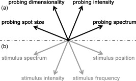 The probing spectrum and probing intensity are among the most influential parameters, as near-infrared light itself, is believed to have a strong effect on the human retina and can cause prestimuli or even eventually saturate the response function of the photoreceptors.2 Because our experiments are performed in the near-infrared region at , our aim must be to use the least probing intensity, keeping potential prestimuli as low as possible, while maintaining high sensitivity. Other research groups suggest using light sources centered at for probing retinal function in order to further separate the stimulation and detection spectra.18 However, extensive studies comparing the spectral influence of the light stimulus in the visible and infrared region on retinal response have not yet been performed. Concerning the stimulus positions, we believe that for future experiments it could be certainly worthwhile to investigate different stimulus regions because the density and distribution of photoreceptors differs drastically throughout the retina. The stimulus and probing position was chosen for the following reasons: first, we tried to keep close distance to the fovea to probe regions of high photoreceptor density. On the other hand, we avoided the excavation of the foveal pit. In this region, slight lateral position changes due to eye motion would result in probing morphologically different retinal cross sections, which is critical for the temporal frequency analysis. We will discuss the influence of probing spot size as well as stimulus intensity in more detail in Sections 2.2.1, 2.2.2. 2.2.1.Probing spot size determinationA highly critical factor, when investigating a response of individual photoreceptors, is the spot size of the probing beam. To study the amount of signal fluctuations due to eye motion, we recorded fast high-resolution volume series of the retina in vivo at an eccentricity of . At this position, it is possible to observe backscattered intensities from individual photoreceptors even without adaptive optics.20, 14, 15 We expected the intensity fluctuations to be smaller if larger spot sizes are used. On the one hand because the spots will cover larger amounts of photoreceptors, and on the other hand, because even in the presence of eye motion the spots will still cover part of the identical region on the retina. As mentioned in Section 2.1, we used an approximate spot size at the retina of for the high transverse resolution measurements (Table 1, setting A). The volumes used to extract the photoreceptor layers consisted of covering a patch on the retina of . They were recorded at a line rate of , resulting in a volume rate of four volumes per second. The fundus projections used for this experiment [Fig. 3 ] were created calculating average intensities in depth of the extracted photoreceptor layers. The large disk in Fig. 3 (yellow) indicates a spot diameter on the retina of , whereas the smaller disk (orange) indicates a spot diameter on the retina of . Because of involuntary eye motion during acquisition, the probing spots illuminate different sites of the retina and thus are displaced relative to the original position [dashed lines in Fig. 3]. In Fig. 3, a microsaccade is indicated by a black arrow. These are very short involuntary motions in the range of . It is an interesting feature that the eye returns close to its initial position after the microsaccade. The short time scale and small amplitude of such a microsaccade has no measurable influence on further analysis. Clearly, the changes in probing position introduce fluctuations of the backscattered intensity, which might obscure intensity changes due to retinal responses to stimuli. To study the amount of fluctuation, we simulated time evolutions of the backscattered intensity from a single spot within the measurement field and averaged over defined spot diameters. Figure 3 shows the respective intensity variations (solid lines) within region of interest (ROI) B indicated in Fig. 3. As background reference, the average intensity over the full fundus projection is plotted (dotted line). Figure 3 shows the standard deviations of the background corrected intensity fluctuations within ROI A and ROI B for spot sizes in the simulation of . For ROI B, the standard deviations for spot sizes of are very close to those of spot size and correspond to a relative intensity change of . In the case of choosing the ROI across a vessel shadow (ROI A), the standard deviations decrease much less for larger spot sizes. The interpretation of this analysis has to be taken with care because signals were added noncoherently. Nevertheless, we are convinced that it gives a reasonable estimate for the actual conditions. Another indicator emphasizing the use of larger spot sizes is a motion analysis tracking the relative displacements of the fundus projections during time. Figure 3 shows the reconstructed motion path by adding the motion vectors within the fundus plane over a time of . It further points out that spot sizes of will lead to a reasonable overlap in the presence of slight involuntary eye motion. This overlap may be interpreted as a measure of coherence or correlation between the measured signals. If the spots do not cover the same patch on the retina over time, then they will lose their correlation. The values will additionally depend on the photoreceptor density for different regions on the retina,21 shown in Fig. 3 (arrow indicates the eccentricity of the measurement site for this experiment). It certainly has to be mentioned that the optimal spot size depends strongly on the volunteer’s ability to keep the eye on the fixation target. Fig. 3Spot-size simulations on photoreceptor level. (a) Three extracted fundus projections of the photoreceptor layers from a continuously recorded volume time series. The black arrow points at a microsaccade. The large disks (blue: ROI A and yellow: ROI B) illustrates a spot diameter on the retina of , smaller spot (orange) indicates a spot diameter on the retina of (ROI A). Dashed lines indicate the original spot location at time . (b) Intensity variations (solid lines) within ROI B, dotted line indicates average intensity over full fundus projections. (c) Standard deviations of the background corrected intensity fluctuations for ROI A&B. (d) Reconstructed motion path within the fundus plane. (e) Approximate cone spacing depending on eccentricity from fovea (following Ref. 16) Arrow indicates actual eccentricity used for the measurement in this study. (Color online only.) 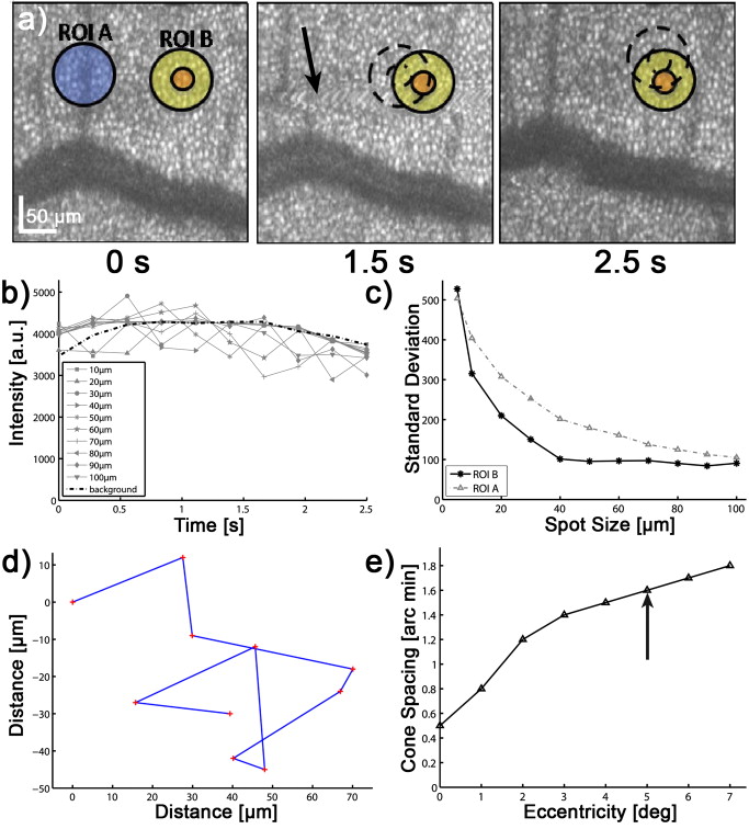 2.2.2.Study of response to single flash stimulusTo find an optimal measurement protocol, we investigated the timing and shape of the response function. We trace the local retinal response at a single spot using an A-scan time series with high temporal sampling of (Table 1, setting B). This line rate has been chosen in order to keep high sensitivity and to be able to compare results to previous studies.22 Furthermore, a sampling rate of is already several magnitudes above the Nyquist frequency of an estimated response in the millisecond range and longer.7 We placed the probing spot on the retina as shown in Fig. 1 and studied responses to single excitation pulses. Figure 4 shows a representative M-scan consisting of 17.000 A-scans over a time of . The synchronization of the system was chosen such that the first of the M-scan serve as the prestimulus baseline. The stimulus lasts for . In order to extract the depth located response signal, the M-scan is flattened to the inner-outer segment photoreceptor (IS/OS) junction using a semi automatic Canny edge algorithm (MATLAB). As indicated in Fig. 4, we calculated the average signal along the depth direction in between the indicated section (red arrows) for each time instant. The extracted section is located just below the strong signal of the IS/OS junction excluding the photoreceptor end tips. The baseline corresponding to the prestimulus average signal was subtracted from the full M-scan. Because we were interested in the retinal response to different stimulus frequencies, we varied the pulse length choosing 25, 50, 125, and . We were able to identify a response signal from the averaged M-scan series for pulse lengths of . This response signature could be reproduced for the same subject, within M-scans that did not suffer from motion artifacts. M-scans containing significant motion artifacts were excluded from the evaluation. They suffer from loss of signal across several retinal layers as well as structural changes. To give an example, Fig. 4 shows a not flattened M-scan with considerable motion artifacts, which was excluded for this study. Figure 4 shows the average plot of the response from the outer photoreceptor segment. Interestingly, we observed a stronger response to the negative stimulus slope that corresponds to switching from light to dark. Figure 4 plots the mean of Fig. 4 over 400 A-scans together with the standard deviation over all averaged M-scans at each time point. Despite the relatively large standard deviations, the shape of the response can be reproduced for independent M-scan series. The recovery slopes after the positive and negative pulse edges were similar in duration of . Considering our frequency-encoded approach, knowledge of this response time and the shape is in fact very important. However, for pulse lengths of , we could not identify a reproducible response signal from the outer photoreceptor segment. The reason for this observation is still unclear and will be investigated in further studies. Also, the probability of finding a clear response signature was . In general, one-point measurements are critically influenced by motion artifacts and by the proper segmentation of photoreceptor layers for signal extraction. Fig. 4Single-point measurements. (a) M-scan suffering from motion artifacts. (b) Flattened M-scan covering . Dotted lines indicate the region where the signal of (c) and (d) is extracted. It is averaged along the depth extend of the box at each lateral position. (c) Signal average for pulse over 5 M-scans. (d) Mean time trace (averaged over 400 A-scans) and standard deviations for the signal in (c). 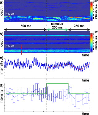 A single response duration of corresponds to a frequency of , which sets an upper limit for the stimulus frequency. Higher frequencies would in principle allow for higher sensitivity by shifting the response signal further away from the dominant 1/f-noise regime. However, they might cause overlap and truncation of the individual response because of their slow decay. 2.3.Frequency-Encoded ApproachOur approach aims at avoiding signal response artifacts due to low-frequency changes. The idea is to record fast B-scan time series across a region of the retina, which is stimulated at a defined frequency with the assumption that any stimulation-induced changes of retinal reflectivity will follow the modulation. The stimulation-induced carrier frequency gives us the important advantage of shifting the detection sensitivity out of the 1/f noise. As we record the B-scan time series across a defined stimulated area on the retina [Fig. 1], we are able to contrast the stimulated against the nonstimulated regions [Fig. 5 ]. Fig. 5Creation of fOCT images. (a) Flowchart of applied data processing. See text for details. (b) Graphic illustration of the fOCT image production. For a registered B-scan series the FFT is calculated for each pixel time trace (left). Yellow flashes symbolize the induced flicker stimulus with a defined frequency, yellow areas within the B-scans indicate the stimulated areas. To each frequency corresponds a functional tomogram that represents the response signal at a specific modulation frequency (right). (Color online only.)  The process to generate fOCT tomograms is outlined in Fig. 5. In order to reveal the reflectivity change, we first perform the fast Fourier transform (FFT) of the recorded spectra with respect to , in order to receive the intensity tomograms . Thereupon, we perform the FFT for each pixel along time to obtain the frequency response or spectral tomograms . The full frequency range is limited by half the B-scan rate according to the Nyquist theorem. The frequency resolution is determined by the temporal length of the time series as . The spectral tomograms are bandpass filtered using a window centered at the stimulus frequency to extract the frequency entry , with being the number of B-scans used for the frequency analysis. The pixels of this frequency response tomogram below a certain threshold are set to transparent. In order to gain information about the change in reflectance relative to the average intensity tomogram along the time coordinate given by , we divide by . The factor of 2 comes from the fact that the amplitude after Fourier transform is divided into positive and negative frequency planes, whereas the dc or zero frequency amplitude remains. In a final step, the frequency response tomogram with color-coded relative change is overlaid to the average intensity tomogram to form a fOCT image. The color-coding outlines regions within the B-scan structure that respond to the stimulus as well as quantifies the relative strength of this response. The B-scan time series require of course proper registration in order to keep the correlation between individual pixels during the time course. For this task, we applied open source ImageJ plug-in software (stackreg), which is based on image correlation,23 originally developed for registering fMRI data. 3.Results and DiscussionThe measurement protocol for producing fOCT maps is as follows: A B-scan time series of 180 B-scans is recorded containing 1000 A-scans each (Table 1, setting C). At an acquisition speed of , the corresponding B-scan sampling rate is . The measurement location has an eccentricity of superior to the fovea [Fig. 1]. The start of the flicker stimulation is triggered by the start of the acquisition. The flicker lasts throughout the complete recording of the 180 B-scans (i.e., for , yielding a frequency resolution of ). On the basis of the results of Section 2.2.1, we chose a beam diameter of . With a flicker frequency of and a duty cycle of 50%, each flicker pulse has a width of . The time period between B-scans of results in 3.4 B-scans per stimulus period. For constructing the fOCT image [Fig. 6 ], we performed the frequency analysis along the time axis and extracted a single spectral tomogram at the expected response frequency [Fig. 6]. Following the procedure of Section 2.2.3 results in the fOCT image of Fig. 6. It represents an overlay of the spectral tomogram [Fig. 6] and the average tomogram [Fig. 6]. We observe a clear signal signature within the stimulated area: the main response originates from the IS/OS junction with spurious responses in the OS photoreceptors. Interestingly, a weak but visible response from the retinal nerve fiber layer is seen. Figure 6 shows the spectral intensity plot of averaged A-scans over a stimulated region (upper blue solid curve) and a plot of averaged A-scans over a nonstimulated region (upper black dotted curve). The regions are indicated in Fig. 6 by the yellow lines for stimulated region and red lines for nonstimulated region. This representation allows for better quantification and gives an estimation of the noise floor. The strongest response is seen at the IS/OS junction with a modulation amplitude of of the average backscattered intensity. For noise floor or background correction, we subtracted the average signal along the frequency coordinate for each pixel resulting in the lower curves for the stimulated (red solid line) and nonstimulated (black dotted line) area in Fig. 6. Another parameter uniquely available through frequency analysis is the phase relation between stimulus and response. Additionally, it may be used to investigate the timing of the responses in the respective retinal structures. The phase difference between stimulus and response is with being the phase offset of the stimulus with respect to . An average plot over 100 adjacent phase depth profiles within the stimulated region is shown in Fig. 6. We observe a significant phase shift with a standard deviation of 0.2 rad. The phase indicates a phase delay of approximately of the response at the IS/OS junction with respect to the periodic stimulus, which in fact strengthens our findings from the single point measurements (Section 2.2.2). This signature has been observed in one out of three volunteers. Fig. 6Results frequency analysis. (a) Average intensity tomogram. (b) Frequency tomogram at . (c) fOCT image for . (d) Spectral intensity over depth, blue solid line: averaged over stimulated region (between yellow lines in (b)); upper black dotted line: nonstimulated region [between red lines in (b)]; red solid line: averaged over stimulated region after background subtraction; lower black dotted line: nonstimulated region after background subtraction; (e) Average phase plot over stimulated region [yellow lines in (b)].  Because responses are of the order of a few percent, it is important to know what determines the spectral noise floor in the frequency representation. Figure 7 shows spectral intensity plots along the frequency axis for structure with high signal-to-noise ratio (SNR) and structure with low SNR differing by . We plotted the noise floors for registered and unregistered time series in order to investigate the effect of correlation loss. As expected, the noise floor increases in the presence of eye motion during the acquisition in particular if the SNR is high (Fig. 7, black dashed line). In contrast high SNR results in a lower noise floor, if the structure during the time course is highly correlated [i.e., with good registration and low motion artifacts (Fig. 7, black solid line)]. This again stresses the importance of proper registration of the image series. Also, choosing the probing region within the foveal pit amplifies the spectral noise floor as the measured structure strongly changes over time in the presence of slight motion. For the case of the low SNR structure, motion artifacts and image registration do not have a large effect on the noise floor (Fig. 7, gray lines), which is nevertheless higher than for the case of better SNR and good correlation. Currently, we use flickering at although slower flicker rate and thus longer pulse duration might increase the response according to our findings in Section 2.2.2. However, the curves of Fig. 7 indicate that switching to slower flicker frequency would critically reduce the advantage of suppressing 1/f noise. Also with our high-speed functional OCT system at hand, which could be used to increase temporal sampling of our signal, we tried as mentioned before to maintain maximum sensitivity by staying with relatively low line rates although higher line rates might help to increase temporal sampling. One could increase the temporal sampling by reducing the numbers of A-scans per B-scan. This might, on the other hand, cause correlation loss along time in the presence of motion due to laterally undersampled speckles. Although we reduce the influence of 1/f noise and increase the specificity of the response detection with the frequency-encoded assessment, there are of course various other factors that influence or might even suppress the response. A possible source of error, which is often underestimated, is the influence of the postprocessing algorithms on the detection of the small changes in backscattered intensity. Our frequency-encoded approach relies on careful registration of B-scans, but spares at least segmentation and flattening of retinal layers. The use of fast retinal tracking could almost entirely eliminate motion artifacts and further enhance the sensitivity of the method. Another issue that has been widely discussed by previous authors is prestimulation of the photoreceptors under investigation. In order to keep the prestimulus low, we introduced precautionary measures: first, we reduced the power of the sampling beam, incident at the cornea to a minimum, and second, we separated the spectrum of the SLD well from the stimulus light. The spectrum of the used light source is located above , where photoreceptors are hardly sensitive; nevertheless, the scanning spot is still slightly visible to the volunteer. Alternatively, one could suppress possible prestimulus by shifting the probing light central wavelength above , which requires a different detector or OCT technology. Furthermore, the volunteer was dark adapted for prior to the experiment. It has been shown by other authors that dark adaption enhances the response signal. A disadvantage of dark adaption might be the unintentional backing off of the volunteer’s head at the initial flash. However, this issue is in our case not as critical because we use a relatively low-power flicker stimulus and take full advantage of the frequency-encoded approach presented in this paper. Even though we discuss several of the most critical artifacts that can easily distort small signals, the list is not meant to be exhaustive. As a final remark, it may be interesting to investigate different stimulus positions as the number of photoreceptors per square millimeter, the ratio of cone/rod photoreceptors or the vascularization throughout the retina differs significantly and therefore may lead to different findings concerning response strength or timing. 4.Conclusion and OutlookWe presented a novel experiment design for the noninvasive assessment of neural retinal tissue function with enhanced sensitivity. By matching the response detection to a defined flicker frequency stimulus similar to heterodyne detection, the response signal will be shifted out of the 1/f noise. Preliminary results prove the feasibility of the measurement concept. Furthermore, we investigated the function and timing of the response function to a single flash stimulus. Gaining knowledge of the exact shape of this function will in the future help to further enhance the sensitivity of our frequency-encoded approach, in particular, if such information is treated with advanced signal-processing tools used in functional magnetic resonance tomography (fMRI), such as wavelet analysis, regression models, or other parametric models used to test the response signals against null hypotheses. Because the retina offers easy access to neuronal tissue, we consider fOCT as a potential tool for providing, in a completely noninvasive way, depth-resolved functional maps similar to fMRI plots, with high spatial as well as temporal resolution. Even if current results need further testing based on a larger ensemble of subjects in order to enhance statistical significance, we are convinced that the method itself shows a new direction for assessing with high sensitivity retinal response signatures. AcknowledgmentsFunds from Swiss National Fonds (SNF Grant No. 205321-109704/1) and the European Framework FP7 (FUN-OCT) are acknowledged. We also thank Theo Lasser for providing equipment, Christoph Pache for technical support, and Dimitri Van De Ville for helpful discussions on signal postprocessing. ReferencesR. W. Rodiek, The first steps in seeing, Sinaur Associates, Sunderland, MA
(1998). Google Scholar
H. H. Harary, J. E. Brown, and L. H. Pinto,
“Rapid light-induced changes in near infrared transmission of rods in bufo marinus,”
Science, 202 1083
–1085
(1978). https://doi.org/10.1126/science.102035 0036-8075 Google Scholar
M. D. Abramoff, Y. H. Kwon, D. Ts’o, P. Soliz, B. Zimmerman, J. Pokorny, and R. Kardon,
“Visual stimulus-induced changes in human near-infrared fundus reflectance,”
Invest. Ophthalmol. Visual Sci., 47 715
–721
(2006). https://doi.org/10.1167/iovs.05-0008 0146-0404 Google Scholar
K. Tsunoda, Y. Oguchi, G. Hanazono, and M. Tanifuji,
“Mapping cone- and rod-induced retinal responsiveness in macaque retina by optical imaging,”
Invest. Ophthalmol. Visual Sci., 45 3820
–3826
(2004). https://doi.org/10.1167/iovs.04-0394 0146-0404 Google Scholar
D. A. Nelson, S. Krupsky, A. Pollack, E. Aloni, M. Belkin, I. Vanzetta, M. Rosner, and A. Grinvald,
“Special report: noninvasive multi-parameter functional optical imaging of the eye,”
Ophth. Surg. Lasers Imaging, 36 57
–66
(2005). Google Scholar
K. Grieve and A. Roorda,
“Intrinsic signals from human cone photoreceptors,”
Invest. Ophthalmol. Visual Sci., 49 713
–719
(2008). https://doi.org/10.1167/iovs.07-0837 0146-0404 Google Scholar
R. S. Jonnal, J. Rha, Y. Zhang, B. Cense, W. Gao, and D. T. Miller,
“In vivo functional imaging of humancone photoreceptors,”
Opt. Express, 15 16141
–16160
(2007). https://doi.org/10.1364/OE.15.016141 1094-4087 Google Scholar
A. F. Fercher, W. Drexler, C. K. Hitzenberger, and T. Lasser,
“Optical coherence tomography—principles and applications,”
Rep. Prog. Phys., 66 239
–303
(2003). https://doi.org/10.1088/0034-4885/66/2/204 0034-4885 Google Scholar
C. E. Riva, S. Harino, R. D. Shonat, and B. L. Petrig,
“Flicker evoked increase in optic nerve head blood flow in anesthesized cats,”
Neurosci. Lett., 128 291
–296
(1991). https://doi.org/10.1016/0304-3940(91)90282-X 0304-3940 Google Scholar
A. Grinvald, R. D. Frostig, E. Lieke, and R. Hildesheim,
“Optical imaging of neuronal-activity,”
Physiol. Rev., 68 1285
–1366
(1988). 0031-9333 Google Scholar
G. A. Borgula, R. H. Steinberg, and C. J. Karowski,
“Light-evoked changes in extracellular pH in frog retina,”
Vision Res., 29 1069
–1077
(1989). https://doi.org/10.1016/0042-6989(89)90054-0 0042-6989 Google Scholar
K. Bizheva, R. Pflug, B. Hermann, B. Povazay, H. Sattmann, P. Qiu, E. Anger, H. Reitsamer, S. Popov, J. R. Taylor, A. Unterhuber, P. Ahnelt, and W. Drexler,
“Optophysiology: Depth-resolved probing of retinal physiology with functional ultrahigh-resolution optical coherence tomography,”
Proc. Natl. Acad. Sci. U.S.A., 103 5066
–5071
(2006). https://doi.org/10.1073/pnas.0506997103 0027-8424 Google Scholar
R. Leitgeb, C. K. Hitzenberger, and A. F. Fercher,
“Performance of Fourier domain vs. time domain optical coherence tomography,”
Opt. Express, 11 889
–894
(2003). https://doi.org/10.1364/OE.11.000889 1094-4087 Google Scholar
B. Potsaid, I. Gorczynska, V. J. Srinivasan, Y. Chen, J. Jiang, A. Cable, and J. G. Fujimoto,
“Ultrahigh speed spectral/Fourier domain OCT ophthalmic imaging at 70,000 to 312,500 axial scans per second,”
Opt. Express, 16 15149
–15169
(2008). https://doi.org/10.1364/OE.16.015149 1094-4087 Google Scholar
T. Schmoll, C. Kolbitsch, and R. A. Leitgeb,
“Ultra-high-speed volumetric tomography of human retinal blood flow,”
Opt. Express, 17 4166
–4176
(2009). https://doi.org/10.1364/OE.17.004166 1094-4087 Google Scholar
V. J. Srinivasan, M. Wojtkowski, J. G. Fujimoto, and J. S. Duker,
“In vivo measurement of retinal physiology with high-speed ultrahigh-resolution optical coherence tomography,”
Opt. Lett., 31 2308
–2310
(2006). https://doi.org/10.1364/OL.31.002308 0146-9592 Google Scholar
V. J. Srinivasan, Y. Chen, J. S. Duker, and J. G. Fujimoto,
“In vivo functional imaging of intrinsic scattering changes in the human retina with high-speed ultrahigh resolution OCT,”
Opt. Express, 17 3861
–3877
(2009). https://doi.org/10.1364/OE.17.003861 1094-4087 Google Scholar
W. Drexler,
“Cellular and functional optical coherence tomography of the human retina the Cogan lecture,”
Invest. Ophthalmol. Visual Sci., 48 5340
–5351
(2007). https://doi.org/10.1167/iovs.07-0895 0146-0404 Google Scholar
R. Leitgeb, W. Drexler, A. Unterhuber, B. Hermann, T. Bajraszewski, T. Le, A. Stingl, and A. Fercher,
“Ultrahigh resolution Fourier domain optical coherence tomography,”
Opt. Express, 12 2156
–2165
(2004). https://doi.org/10.1364/OPEX.12.002156 1094-4087 Google Scholar
M. Pircher, B. Baumann, E. Götzinger, H. Sattmann, and C. K. Hitzenberger,
“Simultaneous SLO/OCT imaging of the human retina with axial eye motion correction,”
Opt. Express, 15 16922
–16932
(2007). https://doi.org/10.1364/OE.15.016922 1094-4087 Google Scholar
Y. Zhang, B. Cense, J. Rha, R. S. Jonnal, W. Gao, R. J. Zawadzki, J. S. Werner, S. Jones, S. Olivier, and D. T. Miller,
“High-speed volumetric imaging of cone photoreceptors with adaptive optics spectral-domain optical coherence tomography,”
Opt. Express, 14 4380
–4394
(2006). https://doi.org/10.1364/OE.14.004380 1094-4087 Google Scholar
R. A. Leitgeb, R. Michaely, A. Bachmann, T. Lasser, and C. Blatter,
“Frequency encoded optical assessment of human retinal physiology,”
Proc. SPIE, 6844 68440I
(2008). https://doi.org/10.1117/12.764330 0277-786X Google Scholar
P. Thévenaz, U. E. Ruttimann, and M. Unser,
“A pyramid approach to subpixel registration based on intensity,”
IEEE Trans. Image Process., 7 27
–41
(1998). https://doi.org/10.1109/83.650848 1057-7149 Google Scholar
|