|
|
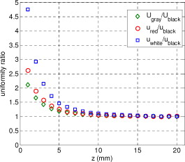
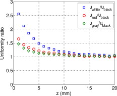
1.IntroductionIn recent years, photoacoustic techniques have demonstrated great potential in a variety of medical applications,1, 2, 3, 4, 5 including imaging brain vasculature,6, 7, 8 ovarian tissue,9 tumor angiogenesis,10, 11, 12 and inflammatory diseases.13, 14 Typical photoacoustic systems employ a short-pulsed laser beam, usually in the near-infrared regime, for tissue irradiation and wideband ultrasound arrays to receive the photoacoustic waves generated by the laser beam upon the absorption of light by tissue. In particular for endoscopic, intravascular, and transvaginal clinical applications, the light delivery is normally accomplished by the use of single or multiple optical fibers in a reflection geometry.18, 19, 20 Two types of ultrasound arrays, namely the linear or phased array and the curved or ring array, are mostly used by research groups to perform photoacoustic imaging. Depending on the ultrasound probe manufacturer, the front face of the ultrasound transducer array is typically a red, gray, or black color, as shown in Fig. 1 , corresponding to different optical reflection coefficients at the irradiation wavelength. In principle, each reflection coefficient of the transducer face enforces a different boundary condition that affects the light fluence and its distribution in a turbid medium. Since the strength of the photoacoustic signal received from the tissue is directly proportional to the light fluence,3 characterizing and understanding the relationship between the boundary conditions and fluence is important to maximize tissue illumination and therefore the signal-to-noise ratio (SNR) of the photoacoustic signal. Additionally, the fluence patterns are required to accurately calculate the quantitative optical properties of heterogeneities via photoacoustic image reconstruction techniques. Fig. 1(a) and (b) Typical curved and (c), (d), and (e) linear ultrasound array transducers used in clinics.  In this work, we have systematically evaluated the light fluence and distribution obtained inside a turbid medium when using each of the three typical ultrasound transducer face colors (gray, black, and red), and compared the results with that obtained using a white color probe of identical size and shape. Monte Carlo (MC) simulations, validated by experiments (Fig. 2 ), were performed to obtain the fluence distribution at various depths inside the turbid medium for each transducer face reflectivity. Section 2 describes the simulation and experimental methods used for these studies. The results are presented in Sec. 3, followed by the discussion and summary in Sec. 4. To the best of our knowledge, our study is the first one to quantify the effects of ultrasound transducer face reflectivity on the light fluence and distribution inside a turbid medium. The result can be used as a reference for irradiation optical design. 2.Methods2.1.Monte Carlo SimulationThe Monte Carlo (MC) technique is a relatively accurate method for modeling light transport in turbid media.15 The optical properties of a turbid medium are described by its absorption coefficient , reduced scattering coefficient , and anisotropy factor . In the MC method, a photon random walk is modeled by statistically sampling the probability distributions of the step size and angular deflection, which follow the exponential and Henyey-Greenstein phase functions, respectively. Briefly, each photon with unity weight is launched into the medium from a source position and moves one step in the direction defined initially by the angle of the light source. Then, for the subsequent steps, the step size and the scattering angle are chosen statistically. For each of these scattering events, a fraction of the photon weight is deposited in each location based on the absorption and scattering coefficients of the medium. The residual photon continues to scatter until it gets either transmitted from the boundaries, or its weight becomes smaller than a predefined threshold. This procedure is repeated for millions of photons, with the accumulated photon weights at each grid element corresponding to the absorbed energy. Finally, the fluence is obtained by dividing the absorbed energy by the local absorption coefficient . In our simulations we considered a semi-infinite medium with a planar boundary. This boundary is perfectly transmitting when the refractive index inside the scattering medium matches that outside. In this case then, the irradiance evaluated at the boundary is zero. On the other hand, if the refractive indices inside and outside the medium are different from each other, then a fraction of the radiant energy incident on the boundary in the scattering medium is reflected back into the medium. This reflected radiance is effectively equivalent to energy from the light source that is incident on the medium Since the angular deflection of photons in the turbid medium is random, the incident angle to the boundary is indiscriminate as well. Therefore, the effective reflection coefficient , representing the fraction of the emittance that is reflected from the boundary and becomes the irradiance, is evaluated for the turbid medium. The value of is obtained by setting the irradiance at the boundary equal to the integral of the reflected radiance16, 17 as whereThe Fresnel reflection coefficient for unpolarized light is defined as: In Eq. 2, and are the refractive indices inside and outside the turbid medium respectively. Also, and are the incident and refracted angles, respectively, and are related to each other by Snell’s law. The parameter is the critical angle for total internal reflection.In photoacoustic imaging, specifically in the reflection mode, the reflection coefficient of the ultrasound transducer face changes the boundary condition, which in turn affects the light fluence distribution inside the medium. The used to model the boundary condition in the simulation was obtained from fitting experimental data. We used this fitting method because of the experimental difficulties arising from measuring the reflection coefficients at various angles, with Intralipid as the surrounding medium. This fitting procedure estimates from the profile of the measured fluence under the center point of the probe versus depth, as explained in Sec. 3 [shown in Fig. 3 ]. Knowing that the peaks of the fluence curves move toward shallower depths with increasing reflection coefficient of the boundary, we accordingly adjusted the refractive index of the boundary until the curve [shown in Fig. 3] fitted that of the experiment. The corresponding was then calculated for each color using Eq. 1. The values were 0.70 for white, 0.45 for red, 0.35 for gray, and 0.00 for black transducer faces. Fig. 3(a) Experimental results, and (b) simulation results of the normalized fluences under the probe center versus depth inside the Intralipid obtained with the four boundary colors.  To simulate the limited numerical aperture of the optical fiber used as a detector in the experiment, as detailed in Sec. 2.2, the same numerical aperture was considered in the simulation. Therefore, the deposition of each photon’s weight in the simulation is recorded per each scattering event only when it is in the range of the fiber’s directional angle. Additionally, the area of the grid elements used to simulate the photon deposition due to absorption was set to to match that of the detecting fiber core used in the experiments. Lastly, the simulations were performed using a tissue sample with optical properties ( , , and ) that correspond to those of the 0.8% Intralipid solution used in the experiments. 2.2.Experimental Setup and MeasurementsThe setup employed for measuring the light fluence distribution with different boundaries is presented in Fig. 2. The measurements were performed in 0.8% Intralipid solution. A Ti-sapphire laser (Symphotics TII, LS-2134) optically pumped by a Q-switched Nd:YAG laser (Symphotics-TII, LS-2122) delivered pulses at with a repetition rate of . The laser beam was coupled into a custom-made high-energy optical splitter assembly (OFS Specialty Photonics) by means of a focusing lens. The assembly features a step-index input fiber and seven multimode output fibers terminated with stainless steel ferrules. Six of the output arms of the splitter were embedded in a flat plate in a circular arrangement of diam and made parallel with the bottom surface of the plate to form the light source. This plate, shown in the inset of Fig. 2, served as a model probe. The seventh output was used for real-time monitoring of the optical energy delivered to the probe. To enable the plate to be moved in precise steps in the , , and directions, it was attached to a PC-controlled motorized 3-D translation stage. The different boundaries were realized by simply pasting colored tapes having the same reflection coefficients as actual clinical ultrasound transducer faces at the bottom and within the fibers. The reflection coefficients of the transducer faces and tapes were measured with the aid of a homemade integrating sphere, as the optical reflections from the faces are diffuse. The sphere comprised two hollow hemispheres, whose insides were coated with silver, joined together to make the sphere. Three holes were made into the sphere; one served as the input for the light, the other served as the output of the diffused light, and the third was used as the insert for the sample, that is, the transducer and tape. The input and insert holes were located such that the incoming light was incident on the sample at a angle. In this way, we were able to measure the approximate reflection coefficients of the transducer faces and tapes that came out as 60% for white, 28% for red, 18% for gray, and 1.4% for black colors at the laser wavelength of . Note that these reflection coefficients measured in free space at only one incident angle of are different from , defined and calculated in Sec. 2. The characterizes the light reflection from a boundary of a diffusive medium, where the incident angle of light is random. The light intensity was measured via a stationary fiber (detector fiber) having a core diameter of and numerical aperture of 0.57. This fiber was securely mounted normal to the plane of the light source and was submerged inside the Intralipid solution. The output end of the detector fiber was then coupled to an optical power meter (Newport 1815-C). Power measurements were recorded on a PC using a data acquisition board (National Instruments PCI 6250) to digitize the analog output signal from the power meter. A LabView program was designed to automate the process of moving the plate and measuring the power. Two sets of experiments were conducted to measure the light fluence distribution. In the first set, the measurements were performed using the aforementioned model probe and changing the boundary reflectivity of the plate as described. In the second set, a real ultrasound transvaginal probe with a gray front face and white edges [Fig. 1] was used. The light fluence distribution, produced by the source fibers surrounding this probe, was measured and compared with the results obtained by using a model probe covered with the gray tape. In all cases, power measurements were performed at four different depths , having values of 5, 10, 15, and below the bottom surface of the plate or probe. At each depth, the fluence distribution was measured by moving the plate or probe in steps of in the plane, covering an area of . 3.Fluence Due to Reflection Coefficient of Transducer Face3.1.Circular ProbeThe experimental results of the fluence distributions obtained with the model probe immersed in Intralipid are shown in Fig. 3 for the white, red, gray, and black boundary colors. Again, these colors correspond to reflection coefficients of 60, 28, 18, and 1.4%, respectively, at wavelength. The fluences shown in both figures were measured [Fig. 3] and computed [Fig. 3] at the center of the probe inside the Intralipid and along the axis in steps below the probe face. In addition, the fluence in each figure has been normalized to the maximum fluence for that figure, which is that obtained with the white-face probe. This normalization provides a convenient way for comparing the four boundary colors. As one would expect, the white-face probe gives the highest fluence when compared to the others, as it has the highest reflection coefficient. At depth, the fluence obtained by using the white-face probe is about six times as great as that obtained with the black-face probe, about three times as large as that obtained with the red-face probe, and about 2.5 times as large as that obtained with the gray-face probe. These values continuously decrease with increasing depth until at about deep inside the Intralipid, when all four boundary colors generate identical fluences. The reason for this is that the photons undergo more scattering as they propagate deep into the scattering medium. Furthermore, it is seen that the fluence curves show peaks where the light beams from the fibers have converged and thus show the highest fluences; these peaks gradually shift toward higher depths with decreasing reflection coefficient from for the white-face to for the black-face probes. Additionally, the peak for the white-face probe is about two times higher than the black-face probe, and 1.5 times higher than the red-face probe, with the gray-face probe in-between. The fluence distributions for the boundary colors are also shown qualitatively in Figs. 4 and 5 for experiment and simulation, respectively. Both are shown within a square area of on the sides and at 5, 10, 15, and depths below the probe face. A comparison of both figures shows good agreement in the fluence distribution profiles of experiment and simulation. The lack of symmetry observed in the fluence distributions for both figures is due to the fact that the output arms of the optical splitter had uneven power distribution. The ratio of the highest to lowest output power of the source fibers was about 1.65 and was taken into account in the simulations. The fluence distributions show that at a depth of , the light beams from the sources have not yet merged, and therefore the central region of the illumination pattern has the least fluence. By depth they have already merged, and from there on the fluence is highest in the center region of the illuminated area where the light beams converge. Comparing the four boundary colors, one observes that the white boundary gives the highest fluence as well as the largest uniformly illuminated area; these effects are even more pronounced around the center regions of the patterns where the light sources converge. Red shows the second highest fluence and second largest uniformly illuminated area at depth. Beyond this depth, however, its performance is comparable to that of gray and black. Clearly as the depth increases from , the uniformity of the fluence distribution also increases for all four boundary colors, as expected. Fig. 4Simulated fluence distribution profiles obtained with white (W), red (R), gray (G), and black (B) color boundaries at (a) 5, (b) 10, (c) 15, and (d) away from the probe and inside the scattering medium.  Fig. 5Experimental fluence distribution profiles obtained with white (W), red (R), gray (G), and black (B) color boundaries at (a) 5, (b) 10, (c) 15, and (d) away from the probe and inside a 0.8% Intralipid solution.  The fluence distribution obtained with the incident light making angles with the probe face was also simulated and compared for the four boundary colors. Xie, Wang, and Zhang already studied the effect of the light source incident angle on the illumination in the dark-field confocal photoacoustic microscopy.21 Here, we investigate the effect of angled light source on the fluence distribution for transducer faces with different reflection coefficients in a bright-field configuration. Figure 6 compares the fluence versus depth under the center of the probe face for the white-face probe to the red-, gray-, and black-boundary colors, and Fig. 7 shows the corresponding qualitative fluence distribution. Figure 6 indicates that at a depth of , the use of the white-face probe provides fluence that is 5.5 times as high as the black-face probe, and drops down to about two times by . Compared with the gray-face probe, the white face is greater by a factor of 2.5 at and about 1.5 by . For the red face, the increment factor is about 2 at and 1.5 by deep inside the turbid medium. In a like manner to the normally incident light-source arrangement in Fig 3, the angled light source also shows a shift in the fluence peaks from for the white-face probe to for the black face. Comparing the peaks, the white-face probe gives about two times as much fluence as the black-face probe, and about 1.5 times as much as the gray- and red-face probes. Fig. 6Normalized fluences under the probe center versus depth obtained with the different boundary colors using angled sources.  Fig. 7Simulated fluence distribution profiles obtained with white (W), red (R), gray (G), and black (B) color boundaries using angles sources at (a) 5, (b) 10, (c) 15, and (d) away from the probe and inside a 0.8% Intralipid solution. 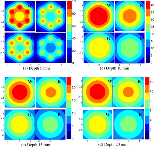 We also performed an experiment to determine the practicality of our model probe comprising the flat plate surrounded by optical fiber (Fig. 2) to mimic an actual ultrasound transducer face. The six optical fibers surrounding the model probe were similarly arranged round a commercial-grade transvaginal probe [shown in Fig. 1] of identical size. The fluence distribution generated by the transvaginal probe was then measured and compared with the fluence generated by the model probe with the gray-colored tape. The result is illustrated in Fig. 8 . As one can see, both the model and actual probes show identical fluence distribution patterns along the axis. Therefore, the use of the model probe to study the effects of boundary conditions of actual transducers on the fluence is appropriate and provides accurate results. Fig. 8Normalized fluence under the center probe versus depth. The red line represents the data obtained by using the gray color-taped model probe (Fig. 2), and the green diamond represents experimental data obtained by using a commercial transvaginal probe with gray color face [Fig. 1]. (Color online only.)  3.2.Linear ProbeFollowing the same approach as the circular probe, fluence distributions were simulated for a rectangular-linear probe having dimensions of . Linear transducer arrays of this dimension are typically used in clinical applications for breast, abdominal, and peripheral imaging. Six light sources were used for the simulation as before, with three on each of the longitudinal sides and equally spaced apart. The fluence along the center of the probe inside the turbid medium at various depths is shown in Fig. 9 . Again, one observes that there is a significant increase in the fluence generated due to the use of the white-face probe compared to the other colors, especially at the shallow depths. This is so despite the relatively larger size of the probe face used here compared with the circular in Sec. 3.1. At a depth of , the white-face probe yields about 4.5-fold increase in the fluence compared to the black, 2.5-fold compared to gray, and two-fold compared to red. These increments in fluence decrease with increasing depth until, at about depth, the fluences are approximately the same. The shifts in the peaks of the fluence curves can also be noticed in the figure. The white-face probe shows a peak at depth and the black-face at . Both the red- and gray-face probes have their peaks at depth. The ratio of the peak fluence of the white-face to the black-face probe is about 1.5, whereas that of the white-face to the red- and gray—probes is about 1.3. These differences in the fluence peaks of the boundary colors are not as significant as in the circular probe due to the larger size of the rectangular probe that was considered here. Fig. 9Normalized fluences under the linear probe center versus depth obtained with the different face reflectivities.  The qualitative fluence distributions for the boundary colors of the linear probe are also shown in Fig. 10 for a square area of at 5, 10, 15 and depths below the probe face. A comparison of the fluence distributions of the white-face to the other three colored-face probes show similar trends, as in the case of the circular probe. 3.3.Uniformity Due to Reflection Coefficient of Transducer FaceA uniformity parameter was introduced to compare the uniformities of the fluences generated by the boundary colors. For a given area, this parameter is defined as the ratio , where is the average fluence, the maximum fluence, and the minimum fluence in that area. 3.3.1.Circular probeThe uniformity parameter obtained for the different boundary colors of the circular probe is shown in Fig. 11 . This parameter was simulated for the plane (lateral uniformity) centered below the probe face within an area measuring . The values of are normalized to that of the black-face probe for easy comparison. Comparing the boundary colors, it is observed that the white-face probe again shows improved uniformity of the fluence generated by a factor of 4.5 over the black-face probe, and about two times as better uniformity as the red- and gray-face probes at depth. As in the case of the fluences, the uniformities of the boundary colors also get closer and closer to each other as the depth increases until about , when they all become indistinguishable. Fig. 11Uniformity parameter simulated for the boundary colors of the circular probe. The values are normalized to the uniformity of the black-face probe. (a) Lateral uniformity in the plane, and (b) longitudinal uniformity in the plane.  The uniformity parameter was also investigated in the longitudinal direction in the plane centered under the circular probe, as shown in Fig. 11. The values of and chosen were ( is the center of the probe face) and , respectively. The highest uniformity occurs in the plane located at , where the white-face probe has about 1.5 times better uniformity than the black-face probe and about 1.2 better than the red- and gray-face probes. Therefore, the choice of boundary color has less influence on the longitudinal uniformity when compared to the lateral uniformity. As mentioned before, the small difference in the longitudinal uniformity between the different color boundaries is due to the fact that scattering effects increase with increasing depth inside the Intralipid. The normalized lateral uniformity was also simulated for the case of the angled sources, and the result is presented in Fig. 12 . The figure indicates that the use of the white-face probe increases the uniformity by a factor of approximately 6 compared to the black-face probe, and by a factor of 2.5 compared to the red-and gray-face probes at depth. This improvement diminishes with increasing depth, until at the uniformities are similar. 3.3.2.Linear probeThe normalized lateral uniformity parameter within a area inside the turbid medium directly below the rectangular-linear probe face is shown in Fig. 13 . Here, the uniformity of the fluence generated by the white-face probe is about 2.5 times more than the black-face probe, and about 1.6 times more than the red- and gray-face probes at depth. By depth, the uniformities of the four boundary colors have gotten close enough to see any appreciable differences. The longitudinal uniformity of the fluence obtained with the rectangular probe was also investigated and was found to be similar to that of the circular probe. 4.Discussion and SummaryA series of experiments and simulations have been performed to investigate the effect of ultrasound transducer face reflectivity on the light fluence distribution for photoacoustic imaging in reflection geometry. Two types of transducer faces were studied. One is the circular or ring-shaped transducer of diam that is normally used in cardiac and transvaginal applications. The other is the rectangular-shaped transducer measuring that is typically used in applications such as breast imaging. The effect of the incident angle on the fluence distribution generated by transducer faces having different reflectivities was also examined. The conclusions drawn from this work are that the use of a highly optically reflecting transducer face provides a substantial increment in the fluence as well as improved uniformity when the imaged tissue is located at a relatively small depth. In the present work, we modeled a 60% reflection coefficient transducer face and compared the fluence it generates with faces having relatively smaller reflection coefficients, which is characteristic of those used in the clinics. It was found that the 60% reflection coefficient face increased the fluence by as much as six times and improved the lateral uniformity by as much as 4.5 times compared to commercially available transducer faces at a depth of around . This improvement, however, gets insignificant by the time the photons reach deep into the turbid medium. Furthermore, it was also found that the use of a angled source yielded identical results as the normally incident source at small depths, but then showed enhanced performance as the depth increased until about depth, where it gave about two times as much fluence and lateral uniformity as the normally incident source. There is no reason why even higher than 60% reflecting surfaces cannot be employed, and it is expected that their use would give more improved results than those reported here. Unfortunately, such optically highly reflecting ultrasound transducer faces are not available on the market and have to be custom-made for photoacoustic applications. We anticipate that with the increasing interest in clinical applications of photoacoustic techniques, ultrasound probe manufactures will consider using high reflection coefficient materials for the front face of their transducers. One option would be to apply a thin coat of water-insoluble white paint, or other kind of solution, on the face of the ultrasound array to achieve the desired reflection coefficient without attenuating the detected photoacoustic signals. In this present work, we investigate the light fluence distribution using typical fatty tissue background optical properties of and . We also evaluate in another work the effect of boundary reflection coefficient using typical muscle and dense tissue background properties of and . When compared with the result obtained by using background properties of soft tissue, the fluence is slightly lower at shallower depths but comparable at deeper ranges. This is because at a shallower depth, the higher background scattering increases the fluence due to increased interaction of photons with the reflective boundary. Therefore, the results reported in this study can be generalized to photoacoustic imaging of biological tissues in the similar range of background optical absorption and scattering properties. AcknowledgmentsWe acknowledge OFS Research Labs and OFS Specialty Photonics for their generous supply of the high-energy optical fiber splitter assembly. We also recognize partial support from NIH (R01EB002136), the Donaghue Research, and Connecticut Breast Health Initiative Incorporated. ReferencesL. V. Wang,
“Prospects of photoacoustic tomography,”
Med. Phys., 35
(12), 5758
–5767
(2008). https://doi.org/10.1118/1.3013698 0094-2405 Google Scholar
L. V. Wang,
“Tutorial on photoacoustic microscopy and computed tomography,”
IEEE J. Sel. Top. Quantum Electron., 14
(1), 171
–179
(2008). https://doi.org/10.1109/JSTQE.2007.913398 1077-260X Google Scholar
M. Xu and L. V. Wang,
“Photoacoustic imaging in biomedicine,”
Rev. Sci. Instrum., 77
(4), 041101
(2006). https://doi.org/10.1063/1.2195024 0034-6748 Google Scholar
R. A. Kruger, D. R. Reinecke, and G. A. Kruger,
“Thermoacoustic computed tomography—technical considerations,”
Med. Phys., 26
(9), 1832
–1837
(1999). https://doi.org/10.1118/1.598688 0094-2405 Google Scholar
A. Oraevsky and A. A. Karabutov,
“Ultimate sensitivity of time-resolved optoacoustic detection,”
Proc. SPIE, 3916 228
–239
(2000). https://doi.org/10.1117/12.386326 0277-786X Google Scholar
J. Gamelin, A. Maurudis, A. Aguirre, F. Huang, P. Guo, L. Wang, and Q. Zhu,
“A real-time photoacoustic tomography system for small animals,”
Opt. Express, 17
(13), 10489
–10498
(2009). https://doi.org/10.1364/OE.17.010489 1094-4087 Google Scholar
J. Gamelin, A. Aguirre, A. Maurudis, F. Huang, D. Castillo, L. V. Wang, and Q. Zhu,
“Curved array photoacoustic tomographic system for small animal imaging,”
J. Biomed. Opt., 13
(2), 024007
(2008). https://doi.org/10.1117/1.2907157 1083-3668 Google Scholar
X. Wang, Y. Pang, G. Ku, X. Xie, G. Stoica, and L. V. Wang,
“Noninvasive laser-induced photoacoustic tomography for structural and functional in vivo imaging of the brain,”
Nature Biotechnol., 21
(7), 803
–806
(2003). https://doi.org/10.1038/nbt839 Google Scholar
A. Aguirre, P. Guo, J. Gamelin, S. Yan, M. M. Sanders, M. Brewer, and Q. Zhu,
“Co-registered three-dimensional ultrasound and photoacoustic imaging system for ovarian tissue characterization,”
J. Biomed. Opt., 14
(5), 054014
(2009). https://doi.org/10.1117/1.3233916 1083-3668 Google Scholar
V. G. Andreev, A. A. Karabutov, S. V. Solomatin, E. V. Savateeva, V. Aleinikov, Y. V. Zhulina, R. D. Fleming, and A. Oraevsky,
“Optoacoustic tomography of breast cancer with arc-array transducer,”
Proc. SPIE, 3916 36
–47
(2000). https://doi.org/10.1117/12.386339 0277-786X Google Scholar
C. G. Hoelen, F. F. de Mul, R. Pongers, and A. Dekker,
“Three-dimensional photoacoustic imaging of blood vessels in tissue,”
Opt. Lett., 23
(8), 648
–650
(1998). https://doi.org/10.1364/OL.23.000648 0146-9592 Google Scholar
J. J. Niederhauser, M. Jaeger, R. Lemor, and P. Weber,
“Combined ultrasound and optoacoustic system for real-time high-contrast vascular imaging in vivo,”
IEEE Trans. Med. Imaging, 24
(4), 436
–440
(2005). https://doi.org/10.1109/TMI.2004.843199 0278-0062 Google Scholar
D. L. Chamberland, J. D. Taurog, J. A. Richardson, and X. Wang,
“Photoacoustic tomography: a new imaging technology for inflammatory arthritis—as applied to tail spondylitis in rats,”
Clin. Exp. Rheumatol., 27
(2), 0387
–0388
(2009). 0392-856X Google Scholar
X. Wang, D. L. Chamberland, and D. A. Jamadar,
“Noninvasive photoacoustic tomography of human peripheral joints toward diagnosis of inflammatory arthritis,”
Opt. Lett., 32
(20), 3002
–3004
(2007). https://doi.org/10.1364/OL.32.003002 0146-9592 Google Scholar
L. Wang, S. L. Jacques, and L. Zheng,
“MCML-Monte Carlo modeling of light transport in multi-layered tissues,”
Comput. Methods Programs Biomed., 47 131
–146
(1995). https://doi.org/10.1016/0169-2607(95)01640-F 0169-2607 Google Scholar
R. C. Haskell, L. Svaasand, T.-T. Tsay, T.–C. Feng, M. S. McAdams, and B. J. Tromberg,
“Boundary conditions for the diffusion equation in radiative transfer,”
J. Opt. Soc. Am. A, 11
(10), 2727
–2741
(1994). https://doi.org/10.1364/JOSAA.11.002727 0740-3232 Google Scholar
J. C. J. Passchens and G. W. T Hooft,
“Influence of boundaries on the imaging of objects in turbid media,”
J. Opt. Soc. Am. A, 15
(7), 1797
–1812
(1998). https://doi.org/10.1364/JOSAA.15.001797 0740-3232 Google Scholar
A. A. Oraevsky, V. G. Andreev, A. A. Karabutov, D. R. Fleming, Z. Gatalica, H. Singh, and R. O. Esenaliev,
“Laser optoacoustic imaging of the breast: detection of cancer angiogenesis,”
Proc. SPIE, 3597 352
–363
(1999). https://doi.org/10.1117/12.356829 0277-786X Google Scholar
R. G. Kolkman, W. Steenbergen, and T. G. van Leeuwen,
“Reflection mode photoacoustic measurement of speed of sound,”
Opt. Express, 15 3291
–3300
(2007). https://doi.org/10.1364/OE.15.003291 1094-4087 Google Scholar
K. Maslov, G. Stoica, and L. V. Wang,
“In vivo dark-field reflection-mode photoacoustic microscopy,”
Opt. Lett., 30
(6), 625
–627
(2005). https://doi.org/10.1364/OL.30.000625 0146-9592 Google Scholar
Z. Xie, L. V. Wang, and H. F. Zhang,
“Optical fluence distribution study in tissue in dark-field confocal photoacoustic microscopy using a modified Monte Carlo convolution method,”
Appl. Opt., 48 3204
–3211
(2009). https://doi.org/10.1364/AO.48.003204 0003-6935 Google Scholar
|