Direct curvature correction for noncontact imaging modalities applied to multispectral imaging

Jana M. Kainerstorfer; Franck Amyot; Martin Ehler; Moinuddin Hassan; Stavros G. Demos; Victor V. Chernomordik; Christoph K. Hitzenberger; Amir H. Gandjbakhche; Giuseppe Rocco Casale

doi:10.1117/1.3470094

1 July 2010 Direct curvature correction for noncontact imaging modalities applied to multispectral imaging

Jana M. Kainerstorfer, Franck Amyot, Martin Ehler, Moinuddin Hassan, Stavros G. Demos, Victor V. Chernomordik, Christoph K. Hitzenberger, Amir H. Gandjbakhche, Giuseppe Rocco Casale

Author Affiliations +

Journal of Biomedical Optics, Vol. 15, Issue 4, 046013 (July 2010). https://doi.org/10.1117/1.3470094

Abstract

Noncontact optical imaging of curved objects can result in strong artifacts due to the object's shape, leading to curvature biased intensity distributions. This artifact can mask variations due to the object's optical properties, and makes reconstruction of optical/physiological properties difficult. In this work we demonstrate a curvature correction method that removes this artifact and recovers the underlying data, without the necessity of measuring the object's shape. This method is applicable to many optical imaging modalities that suffer from shape-based intensity biases. By separating the spatially varying data (e.g., physiological changes) from the background signal (dc component), we show that the curvature can be extracted by either averaging or fitting the rows and columns of the images. Numerical simulations show that our method is equivalent to directly removing the curvature, when the object's shape is known, and accurately recovers the underlying data. Experiments on phantoms validate the numerical results and show that for a given image with 16.5% error due to curvature, the method reduces that error to 1.2%. Finally, diffuse multispectral images are acquired on forearms in vivo. We demonstrate the enhancement in image quality on intensity images, and consequently on reconstruction results of blood volume and oxygenation distributions.

1. Introduction

Over recent years, the unique potential of optical imaging for disease diagnostics and treatment monitoring has become evident. This has resulted in the rapid development of different optical modalities for biomedical imaging. Some of these techniques have been already moved from bench to bedside. Besides the nonionizing nature of optical methods and their relatively cheap implementation, an attractive feature of optical imaging is that it is usually minimally invasive, often being realized as a noncontact imaging technology, e.g., near-infrared fluorescence imaging,¹ colorimetry,^{2, 3} tissue reflectance spectroscopy,⁴ polarization imaging,^{5, 6, 7} Pearson correlation imaging,^{8, 9, 10} and diffuse multispectral imaging.^{11, 12, 13, 14, 15, 16} Though more convenient or even practical for many clinical applications, noncontact imaging can become a quantitative technique, only if data processing adequately takes into account the shape of the target object (e.g., body surface). The bias, introduced into optical images by the surface curvature of the object, can mask real distributions of optical characteristics of the media that characterize the physiological status of the region of interest, making even qualitative assessment impossible without specially developed methods to remove curvature-related image artifacts. An example of the curvature effect can be seen in Figs. 1 and 1 , where we see the distortion of the images due to curvature. The images were acquired by diffuse reflectance imaging at a wavelength of $800 nm$ , and respectively show a volunteer’s forearm and a cylindrical phantom. For comparison, Fig. 1 shows an image of a flat phantom with the same optical properties as the cylindrical one, but no curvature.

Fig. 1

Examples of multispectral intensity images containing the curvature effect are shown. (a) An intensity image of a healthy volunteer’s lower arm, (b) an intensity image of the cylindrical phantom, and (c) the flat phantom. Images shown were taken at a wavelength of $800 nm$ .

When trying to remove the effect of curvature on reflected intensity, two general approaches are possible. Either the object’s shape is being measured and taken into account or the curvature effect, which is the intensity bias, is being extracted. Several methods aimed at curvature artifact correction have been discussed recently in the literature. These approaches include hardware modification, changes in the measurement protocol, and image processing techniques to qualitatively reduce the curvature effect. All these approaches have in common that the shape is being extracted rather than the effect of shape. Westhauser ¹⁷ illuminated the object with fringe patterns and acquired data from three cameras for extracting the surface curvature. Another approach is to use structured light generated by a beamsplitter mounted on a laser diode and reconstruct the surface by an optical triangulation approach.^{18, 19} However, these approaches require hardware modification and additional measurements to extract the shape of the object before extracting and removing the intensity artifacts. Gioux ²⁰ combined phase-shifting profilometry for shape extraction and modulated imaging for optical properties measurements into one single instrument. The same group showed that modulated imaging is a powerful tool for reconstruction of absorption and scattering coefficients and that low spatial frequencies are maximally sensitive to absorption contrast.²¹ The combination of these approaches into one machine does therefore not require any hardware modification, but does still need additional measurements. Another approach was developed by Zeman, which is based on image processing and used for nonquantitative image enhancement.²² This is not a correction model, however, and is not useful for quantitative modeling, as it cannot provide real intensity values. At this time, no techniques, to our knowledge, have been proposed for quantitative curvature extraction and removal in the images that does not involve additional measurements.

In this work we are introducing a correction method that extracts and corrects the curvature intensity bias rather than measuring the shape of the object. It is not dependent on the imaging modality and does not require any additional measurement on the object. To demonstrate and evaluate the method, we are considering the case of diffuse multispectral imaging, which measures the diffuse reflection from the skin using flat light illumination. Spatial frequencies in the data are therefore not sensitive to absorption contrast. This technique is used to reconstruct and map blood volume and blood oxygenation concentrations. The acquired images are often biased by the curvature of the objects.^{11, 12, 13, 14, 15, 16} This problem has to be addressed after acquisition of the images, because clinical protocols typically prohibit patient skin manipulation to flatten the skin surface for curvature removal.

The method we are proposing for extracting and correcting the curvature effect is computationally inexpensive, adding only a few seconds to the analysis, and robust, as we demonstrate in the results in Sec. 4. It is based on the diffuse reflectance images acquired and does not require additional measures of object shape. As it is based on intensity images, it can be applied to any imaging modality that captures diffuse reflectance images. In our approach, the curvature effect can be removed from existing data by either averaging or fitting of the intensity images without direct shape reconstruction. Our goal is to separate the effects of curvature and skin chromophore variations in the images. We demonstrate that the curvature effect can be separated by either averaging or fitting the rows and columns of the image, giving access to the chromophore-dependent variation. Limitations of the method lie in the object’s shape when using the averaging approach and in the choice of fitting function used for the fitting approach. The advantage of this suggested method is not only that no additional measures are necessary, but also that previously collected data can be reanalyzed to remove curvature effects.

To demonstrate the strengths and limitations of the method, we applied it to numerically simulated objects, phantoms, and in vivo data. We would like to point out that the cases presented here are examples for demonstrating the performance of the algorithms, which might differ for different objects imaged. For the interested reader and for trying the method on images of different geometry than described here, the Matlab codes can be obtained from the corresponding author.

In the first part, we show the application of curvature correction in the case of numerically simulated objects. In the second part, we describe phantom experiments performed on cylindrical and flat objects to validate the technique experimentally. Finally, the fitting method is applied using in vivo acquired multispectral images. We demonstrate the enhancement in image quality on raw intensity images and consequently on reconstruction results of blood volume and oxygenation distributions.

2. Materials

2.1.

Instrumentation

A noninvasive, noncontact diffuse reflectance multispectral imaging system was developed in cooperation with Lawrence Livermore National Laboratory (Livermore, California).^{15, 16} Polarized light from a white light source (halogen $150 W$ , Techniquip, Pleasanton, California) is used for flat illumination of the sample imaged. A second polarizer (Optarius, Malmesburg, United Kingdom) is placed before the detection unit, perpendicular to the incident beam polarization, thus guaranteeing diffuse reflectance measurements and removal of specular reflection.⁶

The distance $(h)$ between the sample and detection unit was held constant $(h = 500 mm)$ by using two He-Ne lasers at a fixed angle. The highest point of the sample was placed at the point where the two lasers intersect.

Light is then captured in a charge-coupled device (CCD) camera (Princeton Instruments CCD-612-TKB, Roper Scientific, Tucson, Arizona) after passing consecutively one of six narrow bandpass filters ( $40 - nm$ FWHM, FS40-NIR-I, CVI Laser, Albuquerque, New Mexico) on a filter wheel. Six wavelength images are taken, the wavelengths being 700, 750, 800, 850, 900, and $1000 nm$ . Only the first four wavelengths were used for further analysis to avoid the influence of water and lipid absorption in the reconstruction.

For calibration purposes, images from a 90% reflectance paper (Kodak) are taken. The raw wavelength intensity images are being divided by the normalized intensity distribution from the paper to remove spatial inhomogeneity from the illumination. Spectral inhomogeneity from the source is being corrected for by utilizing the spectral ratio of the six wavelength images of the paper and thus acquiring correction factors.¹⁵ These corrected images are then used for further processing and will be referred to as “raw” intensity images.

2.2.

Reconstruction of Blood Volume and Oxygenation

In vivo data acquired from healthy volunteers’ forearms using diffuse multispectral imaging was used for reconstruction of blood volume and oxygenation. Reconstruction was performed in MATLAB (Math Works, Natick, Massachusetts) by least squares nonlinear fitting of the data to our analytical skin model.¹⁵ Four wavelength $(λ)$ images were used for reconstruction, 700, 750, 800, and $850 nm$ . The analytical skin model used is based on a two-layered structure, the first one being the melanin containing epidermis, the second one being the blood containing dermis. Optical properties of the skin were taken from literature values^{23, 24, 25} and are summarized in Table 1 . Our model is given as:

Eq. 1

I_{e} (x, y, λ) = S \cdot A_{e} {(x, y, λ)}^{2} \cdot A_{d} (x, y, λ) .

Table 1

Optical properties of the skin.

Wavelength (nm)	μdeoxy [mm−1]	μoxy [mm−1]	vm*μmel [mm−1]	μs′ [mm−1]
700	1.068	0.232	1.772	1.912
750	0.788	0.330	1.408	1.606
800	0.478	0.468	1.136	1.372
850	0.424	0.583	0.928	1.190

The attenuation by the epidermis $A_{e}$ is based on Lambert’s law and can be written as:

Eq. 2

A_{e} (λ) = \exp (- μ_{e} . d_{e}) = \exp [- (v_{m} \cdot 0.66 \cdot 10^{11} \cdot λ^{- 3.33} \cdot d_{e})],

where

v_{m}

is the concentration of melanin,

d_{e}

is the thickness of the epidermis, and

μ_{e}

is the absorption coefficient of the epidermis, which is based on the absorption of melanin. The attenuation by the dermis

A_{d}

, which includes the absorption due to blood volume and oxygenation, is based on the analytical solution of photon migration in turbid media based on the random walk theory²⁶ and can be written as:

Eq. 3

A_{d} (λ) = \frac{\exp [- 2 (μ_{d} ∕ μ_{s}^{'})]}{\sqrt{24 (μ_{d} ∕ μ_{s}^{'})}} . {1 - \exp [- \sqrt{24 (μ_{d} ∕ μ_{s}^{'})}]} \approx 1.06 - 1.45 \cdot {(μ_{d} ∕ μ_{s}^{'})}^{0.35},

where

μ_{s}^{'}

is the reduced scattering coefficient and

μ_{d}

is the absorption coefficient of the dermis, defined as:

Eq. 4

μ_{d} = v_{d b} \cdot [(1 - v_{b oxy}) \cdot μ_{deoxy} + (v_{b oxy}) \cdot μ_{oxy}] .

The scaling factor $S$ , blood volume $v_{d b}$ , and blood oxygenation $v_{b oxy}$ are unknown a priori and were solved for.

3. Methods

In this section, we explain in detail our curvature correction method, which uses either averaging of intensity images or fitting of intensity images. Potentially each of these algorithms can be applied. However, depending on the nature of the acquired images, one may provide more accurate results than the other. After this we describe the specific model of skin chromophores incorporated into our diffuse multispectral imaging system. This system provides a good example for using the curvature correction, because it acquires diffuse reflectance images in a noncontact fashion of objects where the curvature effects are expected to be considerable.

3.1.

Curvature Correction

Our curvature correction algorithm is based on extracting the curvature effect on intensity images and does not require additional measures of the shape of the object. It is applicable when the curvature effect is stronger than signals due to intrinsic changes. If the curvature of the object causes intensity variations, which are smaller than intrinsic changes, the curvature effect can be considered negligible. From now on, we refer to these changes as physiological changes, e.g., due to hematological variation. One can consider physiological changes on top of curvature as variations on top of a carrier frequency, much like an AM radio signal. Extracting the curvature is similar to removal of the carrier frequency, which makes the signal (physiologically significant information) available.

The raw detected intensity $I_{r} (x, y)$ , which is the intensity after correcting for spatial and spectral inhomogeneities of illumination at image pixel position $(x, y) ∊ {1, \dots, n} \times {1, \dots, m}$ , where $n$ and $m$ are the total number of pixels in the horizontal and vertical image axis, respectively, and can be described as a function of emitted intensity $[I_{e} (x, y)]$ from the sample surface, the distance of the detector from the object’s surface $[h (x, y)]$ , and the angle between the surface normal of the object and the direction to the detector $[θ (x, y)]$ . Assuming Lambertian reflection, we can write this dependence as

Eq. 5

I_{r} (x, y) = C (x, y) \cdot I_{e} (x, y),

where

C (x, y) = \cos [(x, y)] ∕ h^{2} (x, y)

is the curvature term. The assumption of diffuse reflection is valid for our multispectral imaging system, as the cross-polarizer used removes specular reflection.

Given a separate measure of the surface, one can eliminate the curvature effect directly using this equation. In the absence of such measures, we can extract the curvature by considering it an intensity effect. To do this, we must first recast Eq. 5, separating the background intensity $I_{b}$ (dc component of the signal, constant), and information intensity $I_{d} (x, y)$ (physiologically significant information, spatially varying). This gives us

Eq. 6

I_{r} (x, y) = C (x, y) \cdot [I_{b} + I_{d} (x, y)],

where the background

I_{b}

is independent of

x

and

y

. It turns out that if we assume that the physiological signal

I_{d} (x, y)

is much weaker than the background

I_{b}

[I_{d} (x, y) ⪡ I_{b}]

, where the magnitude of

I_{b}

is in the order of the average image intensity, we can extract and eliminate the curvature effect

C (x, y)

. If this assumption is violated, then the method may perform poorly. We demonstrate in the results in Sec. 4 that the assumption

I_{d} (x, y) ⪡ I_{b}

is valid for our physiological data.

If we further assume that the distance $h (x, y)$ between the camera and the sample is much bigger than the elevation changes of the sample’s surface that is due to the curvature, then $h$ ’s dependency on $x$ and $y$ is negligible. In the following we treat $h$ as a constant height component that we put into $I_{b}$ and $I_{d}$ , such that the curvature term becomes only angle dependent. We can then recast Eq. 6:

Eq. 7

I_{r} (x, y) = C^{'} (x, y) \cdot [I_{b}^{'} + I_{d}^{'} (x, y)],

where

C^{'} (x, y) = \cos [θ (x, y)]

,

I_{b}^{'} = I_{b} ∕ h^{2}

, and

I_{d}^{'} (x, y) = I_{d} (x, y) ∕ h^{2}

, with

I_{b}^{'}

and

I_{d}^{'}

being the background and data signal at height

h

, which is the smallest distance between the surface and camera (highest point of the sample). If the measurement is being focused on this point,

h

corresponds to the focal distance. We developed two different and independent algorithms to extract

C^{'} (x, y)

. The use of one or the other depends on the geometry of the imaged object.

3.1.1.

Known parametric geometries

For our first method we assume that the curvature term $C^{'}$ only changes along the $x$ and $y$ axis, i.e., there are two functions $C_{1}$ and $C_{2}$ that do not have to be further specified, such that

Eq. 8

C^{'} (x, y) \approx C_{1} (x) \cdot C_{2} (y) .

For instance, this assumption holds if the object is cylindrical and aligned to either the $x$ or $y$ axis in the image. This applies to any geometry that can be described in a separable two-part parametric function. We note, however, that this requires knowledge of the underlying geometry; for example, in an elliptical geometry we would need to know its center.

The second assumption that was already mentioned is that the physiological signal is weak compared to the background, i.e.,

Eq. 9

I_{d} (x, y) ⪡ I_{b} .

Moreover, we suppose that there is a point $(x_{0}, y_{0})$ on the surface whose tangent is perpendicular to the image axis. This yields $θ (x_{0}, y_{0}) = 0$ and hence

Eq. 10

\max_{\begin{matrix} x = 1, . ., n \\ y = 1, \dots, m \end{matrix}} [C^{'} (x, y)] = 1 .

This last assumption will be satisfied for almost any geometry of objects imaged.

First, we compute the averages $r_{1} (y)$ and $r_{2} (x)$ of each column and row of $I_{r}$ , respectively, i.e.,

r_{1} (y) ≔ \frac{1}{n} \sum_{x = 1}^{n} I_{r} (x, y), r_{2} (x) = \frac{1}{m} \sum_{y = 1}^{m} I_{r} (x, y) .

We verify in the following that (under the above assumptions) the term

Eq. 11

E (x, y) ≔ \frac{r_{1} (y) \cdot r_{2} (x)}{\max_{y = 1, . ., m} [r_{1} (y)] \cdot \max_{x = 1, . ., n} [r_{2} (x)]}

approximates the curvature term

C' (x, y)

.

To derive $E (x, y) \approx C' (x, y)$ , we first try to estimate the denominator of $E$ . The maximum of $r_{1}$ is

Eq. 12

\max_{y = 1, . ., m} [r_{1} (y)] = \max_{y = 1, . ., m} [\frac{1}{n} \sum_{x = 1}^{n} C^{'} (x, y) I_{b}^{'} + \frac{1}{n} \sum_{x = 1}^{n} C^{'} (x, y) I_{d}^{'} (x, y)] .

By using $0 ⩽ C^{'} (x, y) ⩽ 1$ and $I_{d}^{'} (x, y) ⪡ I_{b}^{'}$ , the term

\frac{1}{n} \sum_{x = 1}^{n} C^{'} (x, y) I_{d}^{'} (x, y)

is negligible in Eq. 12, and we can estimate

\max_{y = 1, . ., m} [r_{1} (y)] \approx I_{b}^{'} \cdot \max_{y = 1, . ., m} [\frac{1}{n} \sum_{x = 1}^{n} C^{'} (x, y)] .

Due to Eq. 8, this finally yields

Eq. 13

\max_{y = 1, . ., m} [r_{1} (y)] \approx I_{b}^{'} \cdot \frac{1}{n} \sum_{x = 1}^{n} C_{1} (x) \cdot \max_{y = 1, . ., m} [C_{2} (y)] .

Analogously, we obtain

Eq. 14

\max_{x = 1, . ., n} [r_{2} (x)] \approx I_{b}^{'} \cdot \frac{1}{m} \sum_{y = 1}^{m} C_{2} (y) \cdot \max_{x = 1, . ., n} [C_{1} (x)] .

Due to Eqs. 8, 10, we have

1 = \max_{\begin{matrix} x = 1, . ., n \\ y = 1, . ., m \end{matrix}} [C^{'} (x, y)] \approx \max_{y = 1, . ., m} [C_{1} (y)] \cdot \max_{x = 1, . ., n} [C_{2} (x)],

and Eqs. 13, 14 then yield that the denominator of

E (x, y)

is approximately given by

Eq. 15

I_{b}^{'} \cdot I_{b}^{'} \cdot \frac{1}{n} \sum_{x = 1}^{n} C_{1} (x) \cdot \frac{1}{m} \sum_{y = 1}^{m} C_{2} (y) .

The numerator

r_{1} (y) \cdot r_{2} (x) = \frac{1}{n} \sum_{x^{'} = 1}^{n} {C^{'} (x^{'}, y) \cdot [I_{b}^{'} + I_{d}^{'} (x^{'}, y)]} \cdot \frac{1}{m} \sum_{y^{'} = 1}^{m} {C^{'} (x, y^{'}) \cdot [I_{b}^{'} + I_{d}^{'} (x, y^{'})]}

can be expanded such that

r_{1} (y) \cdot r_{2} (x) = \frac{1}{n} \cdot \frac{1}{m} \sum_{\begin{matrix} x^{'} = 1 \\ y^{'} = 1 \end{matrix}}^{n, m} C^{'} (x^{'}, y) \cdot I_{b}^{'} \cdot C^{'} (x, y^{'}) \cdot I_{b}^{'} + T (x, y),

where

T

captures the missing terms. The assumption of Eq. 9 implies

\frac{I_{d}^{'} (x, y)}{I_{b}^{'}} = \frac{I_{d} (x, y)}{I_{b}} \approx 0,

which yields

T (x, y) ∕ I_{b}^{'} I_{b}^{'} \approx 0

. This leads to

\frac{r_{1} (y) \cdot r_{2} (x)}{I_{b}^{'} \cdot I_{b}^{'}} \approx \frac{1}{n} \cdot \frac{1}{m} \sum_{\begin{matrix} x^{'} = 1 \\ y^{'} = 1 \end{matrix}}^{n, m} C^{'} (x^{'}, y) \cdot C^{'} (x, y^{'}) \approx \frac{1}{n} \cdot \frac{1}{m} \sum_{\begin{matrix} x^{'} = 1 \\ y^{'} = 1 \end{matrix}}^{n, m} C_{1} (x^{'}) \cdot C_{2} (y) \cdot C_{1} (x) \cdot C_{2} (y^{'}),

where we have used Eq. 4 By combining this with Eqs. 7, 11, we obtain

Eq. 16

E (x, y) \approx \frac{C_{1} (x) \cdot C_{2} (y) \cdot (1 / n) \sum_{x = 1}^{n} C_{1} (x) \cdot (1 / m) \sum_{y = 1}^{m} C_{2} (y)}{(1 / n) \sum_{x = 1}^{n} C_{1} (x) \cdot (1 / m) \sum_{y = 1}^{m} C_{2} (y)} = C_{1} (x) \cdot C_{2} (y) \approx C^{'} (x, y) .

We can now divide $I_{r}$ by $E$ , which gives us the desired

Eq. 17

\frac{I_{r} (x, y)}{E (x, y)} \approx I_{b}^{'} + I_{d}^{'} (x, y) .

The retrieved intensity $I_{e}^{'} = I_{b}^{'} + I_{d}^{'}$ is the emitted intensity at the focal distance $h$ . If different distances are used for multiple samples, one must further calibrate for the $h^{2}$ component of $C (x, y)$ .

A drawback of this approach is its limitation to curvature terms $C^{'} (x, y) \approx C_{1} (x) \cdot C_{2} (y)$ . This condition is violated as soon as the sample has an unknown or complex geometry.

3.1.2.

Generalized geometries

To circumvent the limitation of having a known geometry, we have developed a second numerical method that is based on iterative polynomial fitting of the intensity image. We skip the assumption in Eq. 8, but we keep Eqs. 9, 10. Removal of the data signal $I_{d}^{'} (x, y)$ to retrieve $C^{'} (x, y) \cdot I_{b}^{'}$ is done by local smoothing. A polynomial function is fitted for each row and each column in the image $I_{r}$ using the polyfit function in MATLAB (Math Works, Natick, Massachusetts).

The polynomial function is fitted for each row,

p_{x} (y) = p_{x, α} y^{α} + p_{x, α - 1} y^{α - 1} + \dots . + p_{x, 1} y^{1} + p_{x, 0}, x ∊ {1, \dots, n},

and each column

q_{y} (x) = q_{y, β} x^{β} + q_{y, β - 1} x^{β - 1} + \dots . + q_{y, 1} x^{1} + q_{y, 0}, y ∊ {1, \dots, m},

where

α

and

β

are the polynomial orders. This results in two surface fits of the image. We expect that the spatial average of these 2-D fits gives the first approximation

{[C^{'} (x, y) \cdot I_{b}^{'}]}^{1}

of the background modulated by the curvature, i.e.,

Eq. 18

{[C^{'} (x, y) \cdot I_{b}^{'}]}^{1} ≔ \frac{p_{x} (y) + q_{y} (x)}{2} .

The first fit of the curvature $C^{'} (x, y) \cdot I_{b}^{'}$ provides a reasonable resemblance of the object’s surface, but is still an approximation. In the presence of a spatially varying data signal, the first fit of the curvature will not be smooth. Considering Eq. 18 as a function of the image,

Eq. 19

{[C^{'} (x, y) \cdot I_{b}^{'}]}^{1} = f (I_{r}),

we may iterate the curvature fit using

Eq. 20

{[C^{'} (x, y) \cdot I_{b}^{'}]}^{k} ≔ f {{[C^{'} (x, y) \cdot I_{b}^{'}]}^{k - 1}},

where

k

is the number of iterations. Performing this iterative fitting will smooth the curvature fit and eliminate distortions that might be present in the first fit.

The choice of fitting function used is based on the geometry of the object. Here we are considering a forearm and show in the results in Sec. 4 that a fifth-order polynomial in horizontal and vertical directions fits the data best, and that six iterations were sufficient for the fitting procedure. For consistency, we have used these fitting parameters for all results.

Due to Eqs. 9, 10, the maximum of $I_{r}$ is essentially given by

\max_{\begin{matrix} x = 1, \dots, n \\ y = 1, \dots, m \end{matrix}} [I_{r} (x, y)] \approx I_{b}^{'} \cdot \max_{\begin{matrix} x = 1, \dots, n \\ y = 1, \dots, m \end{matrix}} [C^{'} (x, y)] = I_{b}^{'} .

By assuming that ${[C^{'} (x, y) \cdot I_{b}^{'}]}^{k} \approx C^{'} (x, y) \cdot I_{b}^{'}$ , for $k = 6$ , we can compute

Eq. 21

\frac{{[C^{'} (x, y) \cdot I_{b}^{'}]}^{k}}{\max_{\begin{matrix} x = 1, \dots, n \\ y = 1, \dots, m \end{matrix}} [I_{r} (x, y)]} \approx \frac{C^{'} (x, y) \cdot I_{b}^{'}}{I_{b}^{'}} = C^{'} (x, y) .

The constraint of this method lies in the choice of the fitting function used. Care must be taken that the spatial frequency of the fitting function chosen is lower than that of the signal, or in other words, that the fitting function used does not fit the data. Otherwise, the fitting function used will fit and remove the data content as well. This curve fitting method was evaluated using the numerical simulation and experimental phantom, as well as in vivo data.

3.2.

Numerical Simulation

A data wave was placed on a $50 - mm$ radius cylinder at a distance $400 mm$ away from the detection plane. To test the theory, we used a background (or average) intensity of unit value and applied to it a sine grating signal of amplitude 1% of the background. We tested and compared three approaches: the approach where we have a measured surface (exact kernel), the averaging approach, and fitting model. We used Eq. 6 to create the cylindrical numerical object, and the exact kernel deconvolution inverts Eq. 6 to extract the emitted intensity $I_{e} (x, y)$ with all variables known. The exact kernel is used as a gold standard to compare the averaging and curve fitting method, and is equivalent to having a separate system to measure shape.

As no imaging technique is free of noise, we evaluated the performance of our curvature correction method in the presence of noise. Noise is defined as average white Gaussian noise applied to the final signal (background plus data wave modulated onto the cylinder) with magnitude determined as a percentage of the original data wave.

3.3.

Phantom Experiments

We used a cylindrical tube embedded in blue paper and flat blue paper, which we refer to as cylindrical phantom and flat phantom, respectively. The blue paper used was regular office paper, and several layers of paper were used to avoid any reflected light from the underlying tube. The diameter of the cylinder was $74 mm$ . Structures were introduced by imprinting shaped objects (letters) on the phantoms. We used pencil, and black and red permanent markers, which are referred to as contrast agents. Different contrast agents result into different data to background (dc component) ratios $(I_{d} ∕ I_{b})$ . For these experiments, optical properties of the paper and contrast agents were not known and not relevant. To experimentally test the curvature correction approaches, the quantity to change was the ratio of data to background $(I_{d} ∕ I_{b})$ . To calculate the ratio, we imaged the flat phantom with the same letters imprinted and evaluated the data signal $(I_{d})$ and the background signal $(I_{b})$ by the following equations.

Eq. 22

I_{d} = \frac{\max [I_{e} (x, y)] - \min [I_{e} (x, y)]}{2},

Eq. 23

I_{b} = \frac{\max [I_{e} (x, y)] + \min [I_{e} (x, y)]}{2} .

The ratios $(I_{d} ∕ I_{b})$ for the different contrast agents at wavelength $800 nm$ were 0.73 (black marker), 0.51 (red marker), and 0.39 (pencil).

3.4.

In Vivo Experiments

Multispectral images were taken on healthy volunteers’ forearms. All subjects signed a consent form, which was approved by the Institutional Review Board (IRB) of the National Institutes of Health under protocol 08-CH-0001.

4. Results

4.1.

Numerical Simulation

In Fig. 2 , we show that in the case of a data wave in the form of a sine grating [Fig. 2], superimposed on a cylindrical shape object [created using Eq. 6], [Fig. 2 left] without noise and [Fig. 2 right] with 50% noise, we can recover the data wave using any of the three considered approaches. These approaches are Fig. 2 exact kernel, Fig. 2 averaging, and Fig. 2 curve fitting approach. Figures 2, 2, 2, left side, show the deconvolution without noise, and Figs. 2, 2, 2, middle, show the deconvolution with noise. The middle row of Fig. 2 Shows that in the case of noise, all three models respond to noise in a qualitatively similar manner and allow reliable recovery of the data wave. The point-wise percentage error is shown in the far right column; it is the deconvolved data wave from the middle column minus the data wave from Fig. 2, divided by the data wave. Wherever the data wave is of zero value, the error goes to infinity (division by zero). Remarkably, this shows that all three approaches perform qualitatively equivalently. To demonstrate that the response to noise of the three models is also quantitatively equivalent, we have taken a set of images over a noise range of 1 to 100% (data not shown). Results show that the average error is the same for all approaches over the entire noise range and stays around zero. The normalized standard deviation shows an equivalent linear trend for all three methods and goes from 0.03 at zero noise to 0.537 at 100% noise applied.

Fig. 2

(a) Data wave (a sine grating), superimposed on [(b), left] a cylindrical object without noise and [(b), right] with 50% noise. Three different approaches for curvature removal were tested; (c) exact kernel deconvolution, (d) horizontal and vertical averaging, and (e) curve fitting. Qualitatively all three approaches perform equally well in the noise-free scenario (left), as well as in the noise scenario (middle). The point-wise percentage error for the noise case is shown in the right column.

In Fig. 3 , we assess the dependence of the object’s alignment relative to the horizontal or vertical image axis. The cylindrical numerical object was rotated $90 \deg$ in $5 - \deg$ steps, and the error in reconstruction caused by this rotation was calculated. As expected, the averaging approach depends on the object’s orientation, whereas the curve fitting approach does not. In Fig. 3, we show the effect of varying the radius of the cylinder, therefore the maximum angle theta, while holding the image size constant at $50 mm$ on the error on reconstructed data. The angles evaluated were $25 to 85 \deg$ . The averaging method is not influenced by changes in angle, therefore changes in the curvature, and recovers the data wave accurately in all cases. The curve fitting method shows an exponential increase in error with increasing angles. At $85 \deg$ , the error is 0.47, which is 47 times larger than the data wave. At angles greater $85 \deg$ , the curve fitting approach brakes down and shows a dependence on sampling accuracy. The exponential increase in error can be explained by the fact that a polynomial function cannot fit a cylinder. When excluding high angles $(> 35 \deg)$ , thus only taking a fraction of the cylinder into account, the curve fitting method performs well, with an error smaller than the data wave. For all other numerical simulation results, a radius of $50 mm$ $(30 \deg)$ was used where the error is much smaller than the data wave $(2.6 \times 10^{- 4})$ .

Fig. 3

(a) Error in reconstruction caused by rotation of the object from the image axis. The cylindrical object was rotated $90 \deg$ in $5 - \deg$ steps. The average error in reconstruction is plotted against the angle of rotation for all three methods. The averaging method highly depends on the orientation of the object axis to the image axis, whereas the curve fitting method does not. (b) Error due to varying curvature. There are changes in the radius, therefore maximum angles of the cylinder were evaluated. The error displayed has units of the data signal of the order of 0.01. The curve fitting method shows an error greater than the data for angles between 85 and $35 \deg$ , and breaks down at angles $> 85 \deg$ . At angles smaller than $35 \deg$ , the error is smaller than the data signal. The averaging method is not affected by the angle.

In Fig. 4 , we illustrate a potential limitation of the curve fitting approach. Two columns of images are shown, the left column being the target data wave and the right being the deconvolved data wave. Here we have reduced the spatial frequency (top to bottom) of our sine grating gradually toward a point where the polynomial function used for fitting begins to fit the data wave. In this degenerative case, we know that the model will not hold. This is expected, but as asserted, such cases should not occur in typical biological samples, which is demonstrated in the in vivo result section. In Fig. 4 we provide a quantitative analysis of this effect. The average error in reconstruction is plotted against the number of cycles of the sine grating in the data wave. With increasing number of cycles or spatial frequency, the error in reconstruction for the curve fitting method decreases. As expected, the averaging approach is not affected by the spatial frequency of the data wave.

Fig. 4

(a) Gradual degradation of the curvature correction using the curve fitting approach when data with decreasing spatial frequencies (top to bottom) are applied. The left column shows the data waves and the right column the deconvolved ones. (b) Error in reconstruction caused by low spatial frequencies in data. The dependence of spatial frequency of the data wave for the curve fitting approach is pointed out by plotting the average error in reconstruction against the number of cycles of the sine grating in the data wave. As expected, the averaging approach is not affected by the varying spatial frequency.

Figure 5 shows an assessment of our fundamental assumption that $I_{d} ⪡ I_{b}$ . The percentage error in reconstruction is plotted against the data-to-background ratio. Ratios evaluated were up to 1, where the data equals the background. Physiologically reasonable ratios, assessed by the in vivo results, were on the order of 0.15. As expected, the error increases with increased ratio for the curve fitting method. While the $I_{d} ∕ I_{b}$ ratio is needed for the theoretical derivation, the averaging approach appears unaffected by the $I_{d} ∕ I_{b}$ ratio and performs equivalently to the known geometry model.

Fig. 5

Error in reconstruction caused by increasing data-to-background signal level. The percentage error in reconstruction was plotted against the ratio of data-to-background $(I_{d} ∕ I_{b})$ for all three methods. The percentage error for ratios up to 1 (data equals background) can be seen, where the error increases dramatically as the ratio goes to 1.

With the numerical simulation we have shown that all three approaches of extracting the curvature are equivalent, qualitatively and quantitatively, and can accurately recover the data wave. We showed the dependence of the results on noise and assessed the potential limitations of the numerical approaches.

4.2.

Phantom Experiments

Multispectral images were acquired from a cylindrical and flat phantom with the same optical properties. For illustrative purposes and conciseness, images are only shown at one wavelength $(800 nm)$ . We evaluated the curve fitting approach and we demonstrate the importance of adequate choice of polynomial order for fitting, the qualitative and quantitative recovery of the object shape, as well as the limitations of the algorithm with high background-to-data ratio.

In Fig. 6 we show the effect of polynomial order on fitting quality. An averaged cross section along the cylinder axis after correction can be seen in Fig. 6. Polynomial orders two and three reduce the curvature effect but do not remove it completely at the edges. No significant difference can be seen between order five and six, which both remove the curvature accurately. Minor residuals $(< 2 %)$ can be seen at the edges of the cylinder, which can be explained by the high angular dependence of the object shape at the edges as well as by the fitting function used. A polynomial function cannot fit a circle and breaks down at the edges. We generated L-curves to make a decision of the best choice of polynomial order for fitting. The normalized standard deviation of all six wavelengths images, after correction for each polynomial order, was calculated. The standard deviation for each L curve was normalized against the maximum standard deviation for each wavelength, and the dependence of standard deviation on the polynomial order can be seen in Fig. 6. Based on these L-curves, we chose fifth order polynomials for the curve fitting approach for our case.

Fig. 6

(a) Dependence of polynomial order on the fitting quality. The averaged, normalized cross section through the cylinder (along the $y$ axis) is plotted for each polynomial order tested. Order five and six fit the object shape accurately, leaving only minor residuals $(< 2 %)$ at the edges of the cylinder. (b) shows the dependence of the polynomial order on normalized standard deviation of the curvature corrected cylinder, illustrated by the L-curves.

Figure 7 shows the cylindrical phantom before and Fig. 7 after curvature correction with the curve fitting approach in comparison to Fig. 7 the flat phantom. We demonstrate that our algorithm is capable of removing the curvature effect qualitatively in the comparison of Figs. 7 and 7. In Fig. 7 we illustrate this recovery quantitatively by showing the averaged cross section for Figs. 7, 7, 7 with error-bars given by the standard deviation over all rows. The mean intensities over the entire image area are $68105 \pm 997$ and $65930 \pm 1095$ for the curvature corrected and the flat phantom, respectively. Values are greater than the saturation limit of the $16 -bit$ camera due to calibration for spectral inhomogeneities¹⁵ and due to the curvature correction. Remaining discrepancies between theses numbers can be explained by the fact that we used a cylindrical phantom that cannot be fitted perfectly by a polynomial function. In comparison, the uncorrected phantom mean intensity is $55022 \pm 15760$ . We therefore show that real intensity values can be recovered within 1.2% error, in comparison to 16.5% error before correction

Fig. 7

Curvature correction based on curve fitting on the cylindrical phantom without data content and compared to the flat phantom. (a) shows the curvature uncorrected intensity image, (b) the curvature corrected intensity image, and (c) shows the flat phantom. (d) shows the averaged cross section of (a), (b), and (c) with error bars given by the standard deviation over all rows.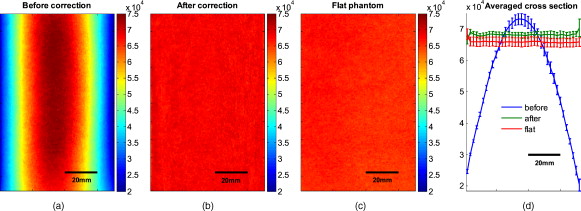

Figure 8 shows the cylindrical phantom with different contrast agents, having decreasing data to background ratios [Figs. 8, 8, 8]. The contrast agents used have different absorption coefficients compared to the background and were therefore used to mimic local changes, which are present for in vivo imaging (vein, hair, lesion, etc.). Different contrast agents were used to see the effect of contrast on the curvature correction. The method used for correction was based on the curve fitting approach. Letters were written perpendicular to the axis of curvature and along it to assess the effect of structure orientation on the curvature correction. Figure 8 shows that for the highest $I_{d} ∕ I_{b}$ ratio (black marker), the least effective curvature correction is achieved. From left to right, Fig. 8 shows the phantom before correction and after correction for letters aligned perpendicular to the curvature, and before and after correction for letters aligned along the curvature. After correction, the remaining curvature is clearly visible in the image area where the letters are written, regardless of orientation. In this case the $I_{d} ∕ I_{b}$ ratio was 0.73 [calculated using Eqs. 22, 23], which is a much higher ratio than physiological changes found in typical biological samples. Qualitative improvement can be seen in Figs. 8 and 8 [ratios 0.51 (red marker) and 0.39 (pencil), respectively], where the algorithm works better as the ratio decreases.

Fig. 8

Curvature correction based on curve fitting on the cylindrical phantom with data (letters). Intensity images are shown before and after curvature correction. Different contrast agents were used with decreasing data-to-background ratios. The different $I_{d} ∕ I_{b}$ ratios are (a) 0.73, (b) 0.51, and (c) 0.39. The figure qualitatively shows the dependence of data-to-background ratio on the correction performance.

The quantitative relationship between the $I_{d} ∕ I_{b}$ ratio and the normalized standard deviation of the curvature corrected image is shown in Fig. 9 . For this comparison, the standard deviation of the background (no letters) was calculated after correction, as it is the background (no letters) that should be equivalent for all contrast agent images. Both cases of feature alignment were considered, perpendicular and along the curvature axis. The descending trend of standard deviation for decreasing ratios is found for both directions of feature alignment. Features aligned along the axis of curvature are less disruptive to the correction than features perpendicular to the curvature axis.

Fig. 9

Dependence of contrast on the curvature correction. The $I_{d} ∕ I_{b}$ ratio is plotted against the normalized standard deviation of the background of the curvature corrected image at a wavelength of $800 nm$ . Both cases of feature alignment are shown, as well as a comparison of the flat phantom without contrast agents.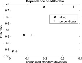

The phantom experiments demonstrated that our algorithm does not only qualitatively remove the curvature, but provides quantitative agreement with flat objects with the same optical properties. We investigated the influence of data-to-background ratio on the correction efficiency, and show that if the ratio is too high, the algorithm may not remove the curvature completely.

4.3.

In Vivo Experiments

We evaluated the curve fitting curvature correction method described in the previous sections using in vivo images taken by our multispectral imaging system. Specifically, using images of a healthy volunteer’s lower arm, we show the improvement in intensity image quality as well as on the reconstruction results for blood volume and oxygenation.

Figure 10 shows the effect of multiple iterations on the curvature fit when using the curve fitting approach. Figure 10 shows a cross section through the curvature fit with veins present. The locations of veins are pointed out by black arrows. The first fit of the curvature is clearly biased by intensity variations due to veins. This effect disappears with increasing number of iterations and the curvature becomes smooth. To quantify this behavior, the squared error of the difference between fits over increasing iterations was calculated, which can be assessed as:

Eq. 24

E_{n} = {{⟨ C^{'} (x, y) \cdot I_{b}^{'} ⟩}^{l - 1} - {⟨ C^{'} (x, y) \cdot I_{b}^{'} ⟩}^{l}}^{2},

where

1 : 2 \to L

, with

L

being the maximum number of iterations. The results of the squared error are shown in Fig. 10. Based on this

L

-curve, we have chosen six iterations for our curvature correction method.

Fig. 10

Effect of multiple iterations on the goodness of fit of curvature is shown in this graph. (a) shows a cross section through the curvature fit for all six iterations. Black arrows indicate the location of veins. It can be seen that the effect of veins disappear after several iterations, leaving a smooth curvature. The L-curve in (b) shows the squared error against number of iterations.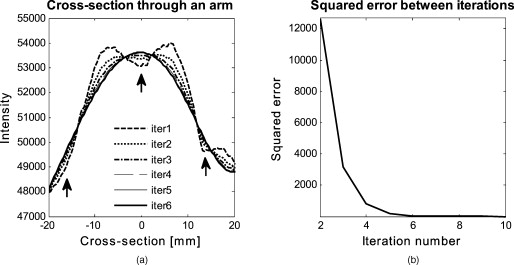

The qualitative improvement of image quality and feature extraction on intensity images for all six wavelengths acquired can be seen in Fig. 11 . Our method is able to recover real intensities, and therefore spectral ratios are retained, which makes further analysis, i.e., reconstruction for blood volume and oxygenation, possible. The curvature corrected images in Fig. 11 were used to evaluate the data-to-background ratios and to confirm that our assumption of $I_{d} ⪡ I_{b}$ holds for our multispectral images. The data signal $(I_{d})$ and the background signal $(I_{b})$ were calculated by Eqs. 22, 23 using the curvature corrected images. We were confident using the corrected images for calculation, as the curvature effect is clearly larger than the data variation, as can best be seen in Figs. 12 and 12 (corrected versus uncorrected). The ratios $(I_{d} ∕ I_{b})$ for all six wavelength images were calculated and were 0.12 $(700 nm)$ , 0.15 $(750 nm)$ , 0.16 $(800 nm)$ , 0.16 $(850 nm)$ , 0.13 $(900 nm)$ , and 0.09 $(1000 nm)$ . Comparing these ratios to the results of the numerical simulation (Fig. 5), a maximum error of 1.2% is expected in the removal of the curvature effect.

Fig. 11

Curvature correction for in vivo data. Intensity images of a healthy volunteer’s arm (a) before and (b) after correction are demonstrated for all six wavelengths. The qualitative enhancement in image quality can be seen in the corrected images.

Fig. 12

Effect of curvature correction on quantification of (a) and (c) fraction blood oxygenation and (b) and (c) fraction blood volume. Reconstruction results (a) and (b) before curvature correction are clearly biased by it. Results after correction (c) and (d) do not show this effect, which can be seen in more detail in the cross sectional plots shown in (e) and (f), with uncorrected in blue and corrected in green. The cross sections shown are indicated by the dotted line in (a). Detailed assessment of tissue chromophore concentration was made possible. (Color online only.)

To assess the improvement on skin chromophore concentrations, image reconstruction for blood volume and oxygenation was performed; representative results are shown in Fig. 12. Reconstruction was performed on uncorrected intensity images and the corresponding curvature corrected ones to evaluate the curvature effect on the reconstruction of chromophore distribution and concentration. Figures 12 and 12 show the reconstruction results for uncorrected images. Almost no structures can be identified, which is even more evident when looking at a cross section through the images, indicated by the dotted line in Fig. 12 and plotted in Figs. 12 and 12. The curvature is clearly visible in both blood oxygenation [Fig. 12] and blood volume maps [Fig. 12]. The effect leads to overestimation of oxygenation in the center of the image and underestimation at the edges; the opposite effect is visible for blood volume. The curvature biases the reconstruction not only toward higher or lower chromophore concentrations, but obscures the structures in the sample imaged. Figures 12 and 12 show the results for curvature corrected images. The overall distribution of chromophore concentration is more uniform and not biased by the curvature anymore. A cross sectional comparison between uncorrected and corrected images can be seen in Figs. 12 and 12. With the curvature correction applied, pixel-wise assessment of chromophore concentration and detailed assessment of small structures was made possible.

We demonstrated the qualitative improvement of curvature correction for multispectral images of in vivo data. The importance of correction becomes evident in the reconstruction results, where the curvature highly biases the spatial distribution of chromophore concentrations and makes pixel-wise assessment impossible. We further demonstrated that detailed feature extraction became possible, allowing assessment of structures over the entire image.

5. Discussion

Direct approaches to curvature correction in noncontact imaging allow us to remove the curvature artifact without extra measurements being required. We present two approaches that can be used in a complementary fashion depending on the imaging paradigm and sample imaged. The performance of the approaches depends on the object images and the spatial extend of the data. Data shown here are therefore seen as examples.

Numerical simulations allowed us to compare the two methods to an exact kernel deconvolution. The exact kernel is equivalent to measuring the geometry precisely with a secondary instrument, and as such it provides a gold standard of the best possible result. We showed that the recovered signal is qualitatively (Fig. 2) and quantitatively equivalent to the exact kernel. Figure 2 illustrates the images recovered from the two methods in the presence of noise, showing qualitative agreement to the exact kernel. We showed that over a range of noise up to 100%, the error in these images is numerically matched to that of the exact kernel. From these results we can assert that the two methods perform with the same quantitative performance as a separate measurement approach. This performance is demonstrated experimentally in Fig. 7, where we recover the intensity value of a curved object to within 1.2% (average over the image); the average error in the uncorrected image is 16%.

The correction of the curvature is achieved by extracting information from the original intensity image. The information is the shape-dependent bias in the image, as described in Eq. 5. We extract this information by one of two methods. The first method is to use an $x ∕ y$ averaging algorithm. This method gives good qualitative and quantitative results, as shown in Fig. 2. However, it is limited by the assumption given in Eq. 8. This constrains us to images with simple geometries aligned to the imaging frame of reference. For the case of generalized geometries, we have developed a curve fitting method as an alternative approach to extract the information. As illustrated in Fig. 3, we see that the averaging method does indeed break down significantly with as little as 5% change in angular orientation to the imaging frame of reference. As expected, our generalized curve fitting model performs equivalently to the exact kernel through all orientations.

Having demonstrated the improvement of the generalized curve fitting approach over the averaging method, we now discuss the limitations of this approach, where the averaging approach may prove more suited to a given curvature correction problem. The first limitation is evidenced in Fig. 3, where we see under areas of high curvature that the curve fitting approach does not recover the background levels as accurately as an exact kernel; however, the averaging approach is unaffected in this case. The second limitation of the curve fitting approach lies in the choice of the fitting function, which has to be chosen carefully, so that it fits the curvature of the object without fitting the spatially varying data signal. The curve fitting method rapidly degenerates both qualitatively [Fig. 4] and quantitatively [Fig. 4] when the spatial frequencies are low. The averaging method is again not affected by such spatial frequency constraints [Fig. 4]. Examples of physiological conditions, for which the described curve fitting method is suitable for, are port wine stains, body parts similar in structure, as described here, wounds, skin lesions, and others. The latter two are suitable conditions to study if they are large compared to the image size and thus occupy most of the image. In general, the curve fitting method, with its parameter as chosen for this presented work, brakes down if features in the image are of low spatial frequency. Examples of those cases could include nevi, lesions if small compared to image size, and others. The final limitation of the curve fitting method is in the $I_{d} ∕ I_{b}$ ratio. Both methods require that $I_{d} ⪡ I_{b}$ and the curvature extraction rapidly degenerates as $| I_{d} | \to | I_{b} |$ (see Fig. 5); no such degeneration is seen for the averaging approach when using a sine grating as data wave.

For the case of multispectral imaging, we wish to choose the most appropriate method. We know that these images can come from any part of the body and therefore the geometry may not be suitable to the averaging method without rotation and image segmentation. This suggests the curve fitting approach would be more suitable; however, we must first consider the other limitations. We know that the spatial variation of the chromophores is high, and that the images will not typically contain high curvature; however, we must consider the ratio $(I_{d} ∕ I_{b})$ . For our in vivo arm data, we found a maximum $I_{d} ∕ I_{b}$ ratio of 0.15, which corresponds to an expected error of 1.2% in recovered signal based on numerical simulation results (Fig. 5). To further validate these numerical results, we tested our imaging system on a cylindrical phantom with imprinted letters (Figs. 8 and 9) to compare the error in recovery. The calculated $I_{d} ∕ I_{b}$ ratios were 0.73 (black marker), 0.51 (red marker), and 0.39 (pencil). A maximum error of 40% was found for black permanent marker (highest ratio), which equates to the expected value from the numerical simulation results with the same ratio. We would like to point out that the phantom experiments with blue paper were not aimed toward mimicking optical properties, rather than mimicking intensity ratios present when different structures with different optical properties are present in the area to be imaged. Due to this, we were able to use paper and markers, which do not have comparable optical properties but do have comparable intensity ratios. For interested readers, we suggest using Eqs. 22, 23 for calculating $I_{d} ∕ I_{b}$ and for putting their work in the same context.

In vivo results demonstrated the importance of curvature correction on identifying underlying tissue structures in the intensity images (Fig. 11) and consequently in the reconstructed blood volume and oxygenation maps (Fig. 12). While the accurate concentrations are unknown due to lack of a control measurement, the curvature effect in the raw images causes distortions in reconstructed maps, leading to physiologically unreasonable over- and underestimation of chromophore concentration. After curvature correction, the chromophore concentrations are more uniform except for areas of different physiology (veins). We demonstrated that the overall spatial distribution is improved over the uncorrected reconstruction results. Pixel-wise comparison between areas was made possible.

6. Conclusion

We introduce a direct, robust, rapid, and elegant methodology to correct for curvature artifacts present in many noncontact optical imaging modalities. The method is based on analysis of raw intensity images by one of two algorithms, either averaging or curve fitting, and does not require any additional measurements of the shape. As no additional data is required, an attractive feature of the method is that already acquired data can be curvature corrected and reanalyzed. The effectiveness of our technique is demonstrated on numerical simulations, phantom experiments, and in vivo data acquired from forearms using multispectral imaging. We evaluate both algorithms in the presence of noise for different angles of sample orientation, for varying curvature, and for varying data signal, either varying in spatial frequency or contrast. Results show that the curvature removal does not bias the recovered signal. They also demonstrate that the curve fitting approach is better for generalized geometries. However, care must be taken regarding degree of curvature, spatial frequency, and data-to-background intensity ratios if this approach is to be chosen over the averaging algorithm. Furthermore, results from phantom experiments show that real intensity values can be recovered, and objects with the same optical properties but different shape can be directly and pixel-wise compared. Based on the numerical simulation results, we find that in the case of in vivo arm data, a maximum error of less than 2% can be expected in the recovery of the signal. We demonstrate the curve fitting approach on in vivo data of the arm for intensity images as well as for reconstruction results of blood volume and oxygenation, and show the importance of taking the curvature into account if pixel-wise assessment of skin chromophores is desired.

Acknowledgments

The research was funded by the Intramural Research Program of the Eunice Kennedy Shriver National Institute of Child Health and Human Development. The Graduate Partnership Program at the National Institutes of Health and the Department of Physics at the University of Vienna in Austria are also acknowledged.

References

1.

J. L. Kovar, M. A. Simpson, A. Schutz-Geschwender, and D. M. Olive, “A systematic approach to the development of fluorescent contrast agents for optical imaging of mouse cancer models,” Anal. Biochem., 367 (1), 1 –12 (2007). https://doi.org/10.1016/j.ab.2007.04.011 0003-2697 Google Scholar

2.

K. Miyamoto, H. Takiwaki, G. G. Hillebrand, and S. Arase, “Development of a digital imaging system for objective measurement of hyperpigmented spots on the face,” Skin Res. Technol., 8 (4), 227 –235 (2002). https://doi.org/10.1034/j.1600-0846.2002.00325.x 0909-752X Google Scholar

3.

J. Pladellorens, A. Pinto, J. Segura, C. Cadevall, J. Anto, J. Pujol, M. Vilaseca, and J. Coll, “A device for the color measurement and detection of spots on the skin,” Skin Res. Technol., 14 (1), 65 –70 (2008). 0909-752X Google Scholar

4.

B. Riordan, S. Sprigle, and M. Linden, “Testing the validity of erythema detection algorithms,” J. Rehabil. Res. Dev., 38 (1), 13 –22 (2001). 0748-7711 Google Scholar

5.

Y. Bae, J. S. Nelson, and B. Jung, “Multimodal facial color imaging modality for objective analysis of skin lesions,” J. Biomed. Opt., 13 (6), 064007 (2008). https://doi.org/10.1117/1.3006056 1083-3668 Google Scholar

6.

S. G. Demos and R. R. Alfano, “Optical polarization imaging,” Appl. Opt., 36 (1), 150 –155 (1997). https://doi.org/10.1364/AO.36.000150 0003-6935 Google Scholar

7.

S. L. Jacques, J. R. Roman, and K. Lee, “Imaging superficial tissues with polarized light,” Lasers Surg. Med., 26 (2), 119 –129 (2000). https://doi.org/10.1002/(SICI)1096-9101(2000)26:2<119::AID-LSM3>3.0.CO;2-Y 0196-8092 Google Scholar

8.

A. Sviridov, V. Chernomordik, M. Hassan, A. Russo, A. Eidsath, P. Smith, and A. H. Gandjbakhche, “Intensity profiles of linearly polarized light backscattered from skin and tissue-like phantoms,” J. Biomed. Opt., 10 (1), 14012 (2005). https://doi.org/10.1117/1.1854677 1083-3668 Google Scholar

9.

A. P. Sviridov, V. Chernomordik, M. Hassan, A. C. Boccara, A. Russo, P. Smith, and A. Gandjbakhche, “Enhancement of hidden structures of early skin fibrosis using polarization degree patterns and Pearson correlation analysis,” J. Biomed. Opt., 10 (5), 051706 (2005). https://doi.org/10.1117/1.2073727 1083-3668 Google Scholar

10.

A. P. Sviridov, Z. Ulissi, V. Chernomordik, M. Hassan, and A. H. Gandjbakhche, “Visualization of biological texture using correlation coefficient images,” J. Biomed. Opt., 11 (6), 060504 (2006). https://doi.org/10.1117/1.2400248 1083-3668 Google Scholar

11.

H. Arimoto, “Multispectral polarization imaging for observing blood oxygen saturation in skin tissue,” Appl. Spectrosc., 60 (4), 459 –464 (2006). https://doi.org/10.1366/000370206776593672 0003-7028 Google Scholar

12.

H. Arimoto, “Estimation of water content distribution in the skin using dualband polarization imaging,” Skin Res. Technol., 13 (1), 49 –54 (2007). https://doi.org/10.1111/j.1600-0846.2006.00188.x 0909-752X Google Scholar

13.

M. Attas, M. Hewko, J. Payette, T. Posthumus, M. Sowa, and H. Mantsch, “Visualization of cutaneous hemoglobin oxygenation and skin hydration using near-infrared spectroscopic imaging,” Skin Res. Technol., 7 (4), 238 –245 (2001). https://doi.org/10.1034/j.1600-0846.2001.70406.x 0909-752X Google Scholar

14.

D. J. Cuccia, F. Bevilacqua, A. J. Durkin, and B. J. Tromberg, “Modulated imaging: quantitative analysis and tomography of turbid media in the spatial-frequency domain,” Opt. Lett., 30 (11), 1354 –1356 (2005). https://doi.org/10.1364/OL.30.001354 0146-9592 Google Scholar

15.

A. Vogel, V. V. Chernomordik, J. D. Riley, M. Hassan, F. Amyot, B. Dasgeb, S. G. Demos, R. Pursley, R. F. Little, R. Yarchoan, Y. Tao, and A. H. Gandjbakhche, “Using noninvasive multispectral imaging to quantitatively assess tissue vasculature,” J. Biomed. Opt., 12 (5), 051604 (2007). https://doi.org/10.1117/1.2801718 1083-3668 Google Scholar

16.

A. Vogel, B. Dasgeb, M. Hassan, F. Amyot, V. Chernomordik, Y. Tao, S. G. Demos, K. Wyvill, K. Aleman, R. Little, R. Yarchoan, and A. H. Gandjbakhche, “Using quantitative imaging techniques to assess vascularity in AIDS-related Kaposi’s sarcoma,” Conf. Proc. IEEE Eng. Med. Biol. Soc., 1 232 –235 (2006). https://doi.org/10.1109/IEMBS.2006.4397377 Google Scholar

17.

M. Westhauser, G. Bischoff, Z. Borocz, J. Kleinheinz, G. von Bally, and D. Dirksen, “Optimizing color reproduction of a topometric measurement system for medical applications,” Med. Eng. Phys., 30 (8), 1065 –1070 (2008). https://doi.org/10.1016/j.medengphy.2007.12.014 1350-4533 Google Scholar

18.

V. Paquit, J. R. Price, F. MeÌriaudeau, K. W. Tobin, and T. L. Ferrell, “Combining near-infrared illuminants to optimize venous imaging,” Proc. SPIE, 6509 6509OH (2007). 0277-786X Google Scholar

19.

V. Paquit, J. R. Price, R. Seulin, F. MeÌriaudeau, R. H. Farahi, K. W. Tobin, and T. L. Ferrell, “Near-infrared imaging and structured light ranging for automatic catheter insertion,” Proc. SPIE, 6141 6141IT (2006). 0277-786X Google Scholar

20.

S. Gioux, A. Mazhar, D. J. Cuccia, A. J. Durkin, B. J. Tromberg, and J. V. Frangioni, “Three-dimensional surface profile intensity correction for spatially modulated imaging,” J. Biomed. Opt., 14 (3), 034045 (2009). https://doi.org/10.1117/1.3156840 1083-3668 Google Scholar

21.

D. J. Cuccia, F. Bevilacqua, A. J. Durkin, F. R. Ayers, and B. J. Tromberg, “Quantitation and mapping of tissue optical properties using modulated imaging,” J. Biomed. Opt., 14 (2), 024012 (2009). https://doi.org/10.1117/1.3088140 1083-3668 Google Scholar

22.

H. D. Zeman, G. Lovhoiden, C. Vrancken, and R. K. Danish, “Prototype vein contrast enhancer,” Opt. Eng., 44 (8), 086401 (2005). https://doi.org/10.1117/1.2009763 0091-3286 Google Scholar

23.

S. L. Jacques, “Skin optics,” Oregon Medical Laser Center News, (1998) http://omlc.ogi.edu/news/jan98/skinoptics.html Google Scholar

24.

I. V. Meglinski and S. J. Matcher, “Quantitative assessment of skin layers absorption and skin reflectance spectra simulation in the visible and near-infrared spectral regions,” Physiol. Meas, 23 (4), 741 –753 (2002). https://doi.org/10.1088/0967-3334/23/4/312 0967-3334 Google Scholar

25.

S. Prahl, “Skin optics,” Oregon Medical Laser Center News, (1998) http://omlc.ogi.edu/spectra/hemoglobin/index.html Google Scholar

26.

A. H. Gandjbakhche and G. H. Weiss, “Random walk and diffusion-like models of photon migration in turbid media,” Prog. Opt., 34 (5), 335 –402 (1995). 0079-6638 Google Scholar

Citation Download Citation

Jana M. Kainerstorfer, Franck Amyot, Martin Ehler, Moinuddin Hassan, Stavros G. Demos, Victor V. Chernomordik, Christoph K. Hitzenberger, Amir H. Gandjbakhche, and Giuseppe Rocco Casale "Direct curvature correction for noncontact imaging modalities applied to multispectral imaging," Journal of Biomedical Optics 15(4), 046013 (1 July 2010). https://doi.org/10.1117/1.3470094

Published: 1 July 2010

Access the abstract

JOURNAL ARTICLE
14 PAGES

DOWNLOAD PAPER SAVE TO MY LIBRARY

GET CITATION

CITATIONS

Cited by 42 scholarly publications and 1 patent.

Explore citations on Lens.org

RIGHTS & PERMISSIONS

Get copyright permission Get copyright permission on Copyright Marketplace

KEYWORDS

Multispectral imaging

Blood

In vivo imaging

Spatial frequencies

Chromophores

Numerical simulations

Optical properties

1.

Introduction

Fig. 1

2.

Materials

2.1.

Instrumentation

2.2.

Reconstruction of Blood Volume and Oxygenation

Eq. 1

Table 1

Eq. 2

Eq. 3

Eq. 4

3.

Methods

3.1.

Curvature Correction

Eq. 5

Eq. 6

Eq. 7

3.1.1.

Known parametric geometries

Eq. 8

Eq. 9

Eq. 10

Eq. 11

Eq. 12

Eq. 13

Eq. 14

Eq. 15

Eq. 16

Eq. 17

3.1.2.

Generalized geometries

Eq. 18

Eq. 19

Eq. 20

Eq. 21

3.2.

Numerical Simulation

3.3.

Phantom Experiments

Eq. 22

Eq. 23

3.4.

In Vivo Experiments

4.

Results

4.1.

Numerical Simulation

Fig. 2

Fig. 3

Fig. 4

Fig. 5

4.2.

Phantom Experiments

Fig. 6

Fig. 7

Fig. 8

Fig. 9

4.3.

In Vivo Experiments

Eq. 24

Fig. 10

Fig. 11

Fig. 12

5.

Discussion

6.

Conclusion

Acknowledgments

References

Show All Keywords

Keywords/Phrases

Search In:

Publication Years