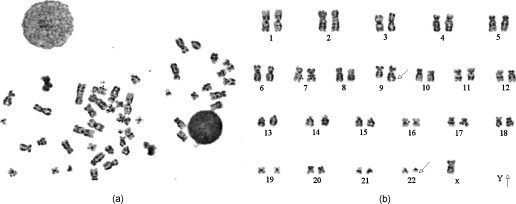
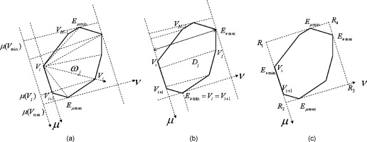
1.

Introduction

Since chromosomal abnormalities are powerful biomarkers in the detection and diagnosis of cancers and other genetic diseases, visualization and classification of metaphase chromosome cells into standard classes (karyotyping) is a fundamental clinical procedure performed in genetic laboratories. A normal metaphase cell includes 46 chromosomes that are grouped into homologous pairs (or classes) 1 to 22 as well as a sex chromosome pair of either XX for a female or XY for a male.¹ Karyotyping aims to identify individual chromosomes in a metaphase cell and arrange them in order based on the established atlas.² In 1960, Nowell and Hungerford³ described a unique and consistent abnormal pattern in chronic myeloid leukemia (CML) patients in which one chromosome 9 and one chromosome 22 swap genes between each other [named a $t(9;22)$ translocation]. Thus, the metaphase cell obtained from a CML patient only has one normal chromosome 9 and one normal chromosome 22. CML is also one of the four common types of leukemia with a poor prognosis.⁴ Hence, early detection and diagnosis of CML is clinically important for optimal treatment of patients to reduce the mortality rate.

Figure 1 shows an example of an analyzable metaphase cell [Fig. 1] selected from a bone marrow specimen. After karyotyping the metaphase cell [Fig. 1], a $t(9;22)$ translocation was discovered and the patient was diagnosed with CML. To show the details of this translocation, the ideogram of these two chromosome classes (9 and 22) are displayed in Figs. 2 and 2 , respectively. As seen in Fig. 2, a piece of chromosome 22 (band q11) breaks, involving a breakpoint cluster region (BCR) gene and attaching to chromosome 9. Similarly, some parts of chromosome 9 (band q34), involving a gene called the Abelson (ABL) gene, attaches to chromosome 22. This translocation makes chromosome 9 longer and shortens chromosome 22 The BCR and ABL genes are⁵ fused together into what is called the BCR-ABL cancer gene causing CML.

Fig. 1

Example of (a) an analyzable metaphase cell and (b) the corresponding karyotyped image.

Fig. 2

(a) Ideogram of chromosomes 9 and 22, (b) special translocation between chromosome 9 and 22, and (c) Philadelphia chromosome in $t(9;22)$ translocations.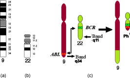

Although karyotyping is a key process for cytogenetic diagnosis of cancers and genetic disorders, visual karyotyping is very tedious and time-consuming. It also introduces substantial interobserver variability. Thus, developing automated karyotyping schemes has been attracting research interests.² In the last $30\mathrm{years}$ , the efforts in developing automated karyotyping schemes primarily focused on the classification of chromosome classes by assuming that all individual chromosomes in a cell have been presegmented. Thus, a set of image features was extracted and different machine learning classifiers including artificial neural networks,^{6, 7, 8, 9} statistical models,^{10, 11, 12, 13, 14} a genetic algorithm,¹⁵ knowledge-based expert schemes,^{16, 17, 18} a transportation algorithm,¹⁹ a homologue-matching algorithm,²⁰ and a fuzzy-logic based classifier²¹ were developed and tested. For example, one study compared the performance of a neural network and a maximum-likelihood-model-based classifier using the same data set and reported²² similar classification accuracy rates of 82.8% (for the neural network) and 81.7% (for the maximum likelihood model). Since the performance of computerized schemes depends on difficult levels of the testing datasets,²³ another study compared the classification performance of a neural-network-based scheme using three publicly available databases with different difficult levels. The study reported the classification error rates of 6.2, 17.8, and 22.7%, when applying the scheme to Copenhagen, Edinburgh, and Philadelphia databases, respectively.²⁴ A previous study²⁵ also showed that by reducing the network size (i.e., the number of hidden neurons), the testing accuracy rate on the chromosome classification increased from 75.8 to 88.3%. In our own previous study,¹⁵ we developed an adaptively optimized neural-network-based two-layer decision tree classifier. When applying it to identify and classify chromosomes in 150 metaphase cells, the classification accuracy rates varied in different classes of the chromosomes ranging from 67.5 to 97.5% (with the overall accuracy rate of 86.8%).

Despite the previous research efforts and the reported progress, most schemes were trained and tested with limited data sets, including normal metaphase chromosome cells extracted from nondiseased specimens. All individual chromosomes have been presegmented (manually or semiautomatically). However, the chromosomes overlapping with each other in the metaphase cells obtained from clinical specimens is often unavoidable. Automatically identifying and segmenting the overlapped chromosomes remains an unsolved technical challenge.²⁶ As a result, it still requires substantial human efforts to sort individual chromosomes and visually correct karyotyping errors when using computerized schemes in the clinical practice.² Since the most recognized genetic abnormalities or diseases have specific numerical/structure changes of only a few chromosomes, identifying such changes is actually the key factor in detecting these abnormalities and helping clinicians make the correct diagnostic decision. Hence, apart from developing the schemes for automated karyotyping, some researchers have focused on developing schemes to detect specific classes of chromosomes without performing the complete karyotyping.²⁷ For example, one research group developed a computerized scheme targeted to detect acute promyelocytic leukemia (APL) that is associated with the distortions in chromosomes 15 and 17. The scheme applied a data-driven homologue-matching algorithm to identify chromosomes of class 17. If the scheme was unable to identify two normal chromosomes 17 in a metaphase cell, the cell was classified as positive for APL. Using a testing dataset involving 55 metaphase cells, the study reported 89.1 and 85.5% cell classification accuracy by using the features extracted from either the density profile or the binary band segmentation profile, respectively.²⁸

In this study, we developed and tested a new computerized scheme to automatically detect and identify normal chromosomes of class 22 using a clinical image data set of bone marrow specimens. Our hypothesis is that if a cell has only one normal chromosome 22, it is highly suspicious for CML and a warning signal should be flagged. The clinicians should pay more attention to examine the case involving the abnormal cell. Therefore, the purpose of this study is to test whether a computerized scheme can automatically prescreen and identify which cases are suspicious for CML with high accuracy.

2.

Material and Methods

In this study, a computerized scheme was developed to identify suspicious metaphase cells that may be associated with a specific type of leukemia (CML), in which one of the two chromosomes in class 22 either has the $t(9;22)$ translocation or is missing. For this purpose, our strategy is to detect and identify whether the cell contains two normal chromosomes in class 22. If the scheme detects either none or only one normal chromosome 22 in a metaphase cell, this cell is flagged as suspicious for being associated with CML. Figure 3 shows a flow diagram of each step of our scheme. Following are the detailed descriptions of our image data set and the steps of the scheme.

Fig. 3

Flow diagram of our computerized scheme to detect and identify chromosomes in class 22.

2.3.

Processing Individual Chromosomes and Feature Extraction

The second step of the scheme is to search for and identify the initial candidates for chromosome 22. Since chromosome 22 is a relatively short chromosome, our scheme first identifies the candidates for chromosome 22 using a simple length criterion to eliminate all chromosomes with relatively longer length (longer than a preestablished threshold). In our experiment, we measured the length of all chromosomes of class 22 in the images of our data set and set up the threshold as 125% of the maximum length of the measurement. To classify whether these selected candidates are true chromosomes of class 22, not other types of short chromosomes or broken parts of long chromosomes, a set of image features must be extracted and computed from each initially selected candidate. Before computing image features from three profiles described later in this section, the scheme must perform several additional steps to define the principal axis of a chromosome and align the axis in the vertical $\left(y\right)$ direction through chromosome rotation. Since the procedure of defining the principal axis and the axis rotation can be applied to all chromosomes in a metaphase cell (not being limited only to chromosome 22), to better illustrate this process in the following descriptions, we selected the longer chromosome 3 as an example (Fig. 4 ).

Fig. 4

Example of finding a minimum enclosing rectangle of a chromosome: (a) an original chromosome, (b) the contour of the chromosome detected by a Sobel filter, and (c) the convex polygon obtained by the Graham scan.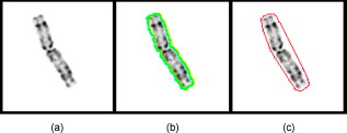

2.3.1.

Identifying a convex polygon using a Graham scan

The scheme uses a Sobel filter to detect the contour of each segmented and selected chromosome [Fig. 4] and records the corresponding locations of the contour points [Fig. 4]. After detecting the contour points of the chromosome, the convex polygon is computed using a Graham scan.³³ After the Graham scan, the vertices of this convex polygon must be identified and recorded. For each point $P$ , the slopes between the previous point and the next point are calculated. If these two slopes are the same, $P$ will be deleted. Figure 4 is the output of a convex polygon of the chromosome [Fig. 4] after implementing the Graham scan and vertex search.

2.3.2.

Searching for a minimum enclosing rectangle for the convex polygon

In the next step, the scheme identifies a minimum enclosing rectangle (MER) for the defined convex polygon. For this purpose, Toussaint³⁴ proposed an algorithm to search for MER by rotating calipers. First, it computes a new set of angles between four sides of the polygon and a rectangle that passes through all these four vertices. Then, the procedure is repeated to search for the rectangle until it has scanned the entire convex polygon. Based on the same theory that the MER for a convex hull has a side collinear with one of the edges of the polygon, we proposed and tested a new MER-searching algorithm with improved computational efficiency by substantially reducing the searching points on the defined convex polygon. The algorithm includes the following steps:

• 1. The scheme searches for the initial four extreme points along both the $x$ and $y$ directions of the convex polygon, which are recorded as $x_{\max }$ , $x_{\min }$ , $y_{\max }$ , and $y_{\min }$ . It constructs a rectangle composed of four lines through these extreme points. The beginning point is $V_0$ with the minimum value $x_{\min }$ in the $x$ direction. Figure 5 displays the rectangle obtained by the initial four extreme points.

• 2. The scheme defines two vectors $\mathbf{\mu }$ and $\mathbf{\nu }$ [as shown in Fig. 6 ]. Vector $\mathbf{\mu }$ is constructed from point $V_i$ to $V_{i+1}$ , $i=0,\dots ,i_{\text{stop}}$ , and the vector $\mathbf{\nu }$ is perpendicular to the $\mathbf{\mu }$ vector. The scheme searches for the four new extreme points along the $\mathbf{\mu }$ and $\mathbf{\nu }$ directions to obtain a new MER.

• 3. The scheme searches for two new extreme points $E_{\mathbf{\mu }\max }$ and $E_{\mathbf{\mu }\min }$ along the $\mathbf{\mu }$ -positive direction [Fig. 6]. Let ${\mathbf{\omega }}_j$ be a vector that is constructed from the point $V_j(j=0,\dots ,N-1,j\ne i,j\ne i+1)$ to $V_i$ , and $\mathbf{\mu }\left(V_j\right)$ is the orthogonal projection of the point $V_j$ projected onto the vector $\mathbf{\mu }$ . Two extreme points can be found by utilizing the following pseudocode: Input $E_{\mathbf{\mu }\max }=E_{\mathbf{\mu }\min }=0$ ; for the point $V_j$ , $(j=0,\dots ,N-1,j\ne i,j\ne i+1)$ . If $\mathbf{\mu }\mathbf{\cdot }{\mathbf{\omega }}_j>E_{\mathbf{\mu }\max }$ , then $E_{\mathbf{\mu }\max }=V_j$ ; If $\mathbf{\mu }\mathbf{\cdot }{\mathbf{\omega }}_j<$ $E_{\mathbf{\mu }\min }$ , then $E_{\mathbf{\mu }\min }=V_j$ .

• 4. The scheme searches for another two extreme points $E_{\mathbf{\nu }\max }$ and $E_{\mathbf{\nu }\min }$ along the $\mathbf{\nu }$ -positive direction [Fig. 6]. Since the rectangle always coincides with the line $V_i$ to $V_{i+1}$ , $E_{\mathbf{\nu }\min }=V_i=V_{i+1}$ . The pseudo code to search for the maximum point $E_{\mathbf{\nu }\max }$ is: For each point $V_j(x_j,y_j)$ , $(j=0,\dots ,N-1,j\ne i,j\ne i+1)$ , calculate the distance between $V_j(x_j,y_j)$ to the vector $\mathbf{\mu }$ . Input $D_{\max }=0$ ; If $D_j=|m_1{x}_j-y_j+d_1|∕{(m_1^2+1)}^{1∕2}>D_{\max }$ , then $E_{\mathbf{\nu }\max }=V_j$ , in which $m_1=(y_{i+1}-y_i)∕(x_{i+1}-x_i)$ , $d_1=y_i-x_i\times (y_{i+1}-y_i)∕(x_{i+1}-x_i)$ .

• 5. The scheme constructs a new rectangle from the detected four extreme points in both the $\mathbf{\mu }$ and $\mathbf{\nu }$ directions. The lines of this rectangle are parallel to the directions of two vectors $\mathbf{\mu }$ and $\mathbf{\nu }$ . One side of this rectangle coincides with the line composed of $V_i$ and $V_{i+1}$ . The scheme computes the area of a new rectangle: ${\mathit{\text{Area}}}_N=[\mathbf{\mu }∕|\mathbf{\mu }|\mathbf{\cdot }{E}_{\mathbf{\mu }\max }-(\mathbf{\mu }∕|\mathbf{\mu }\left|\right)\mathbf{\cdot }{E}_{\mathbf{\mu }\min }]\times D_{\max }$ . Figure 5 is a rectangle and one of its lines is constructed by $V_0$ and $V_1$ .

• 6. If the area of the new rectangle is smaller than the old area, the scheme keeps the current rectangle and deletes the old one. The scheme further rotates the rectangle in the counterclockwise direction.

• 7. The scheme repeats steps 3 to 6 until the rectangle has been rotated $180\mathrm{deg}$ . The rectangle with the minimum area is selected as the final minimum enclosing rectangle for a convex polygon. Figure 5 is the finally identified MER to cover the chromosome.

Fig. 5

(a) Initial rectangle constructed from the initial four extreme points in both the $x$ and $y$ directions, (b) an example of rotating the rectangle found in the first step by using the $\mathbf{\mu }$ direction composed by $V_0$ and $V_1$ , (c) the final minimum enclosing rectangle of the chromosome, and (d) the final rotated chromosome.

Fig. 6

Constructing a rectangle by four extreme points in the $\mathbf{\mu }$ and $\mathbf{\nu }$ directions: (a) searching two extreme points in the $\mathbf{\mu }$ direction, (b) searching two extreme points in the $\mathbf{\nu }$ direction, and (c) constructing a rectangle from four new extreme points.

2.3.3.

Feature extractions

After the MER is obtained, the scheme rotates the chromosome to make its principal axis parallel to the $y$ axis. A detailed description of computing the principle axis was reported in our previous study.³⁵ Figure 5 shows the aligned chromosome after the automated rotation process. After rotation, a segmented chromosome is aligned in the vertical position and its principal axis is calculated. The scheme then extracts and computes chromosome image features based on three profiles, namely, the density, shape, and banding profile. Each profile defines a 1-D graph of a rotated chromosome computed at a sequence of points along the principal axis. The density profile is calculated as $D\left(x\right)=\left[{\sum }_{i=1}^n{g}_i\left(x\right)\right]∕n$ , where $g_i\left(x\right)$ is the gray value of the chromosome projected on the principal axis, and $n$ is the number of all pixels in each perpendicular line. Shape profile $S\left(x\right)=n$ is the number of all pixels in each perpendicular line of the principal axis of the chromosome. A banding profile is computed by processing a density profile $D\left(x\right)$ with a nonlinear transform filter defined by the Kramer and Bruckner method.³⁶ In this profile, each band is characterized by a uniform density and the transitions between neighboring bands are defined as the step functions.³⁷ By assuming that $x$ is the index number of a profile, $B\left(x\right)$ is an original banding profile obtained by a median filtered density profile, $\mathrm{IB}\left(x\right)$ is an idealized banding profile, $\mathrm{NF}\left[B\left(x\right)\right]$ is a nonlinear filter for $B\left(x\right)$ , and $N\left(x\right)$ is neighborhood of $B\left(x\right)$ . We can be compute $\mathrm{IB}\left(x\right)$ using the following equations:

Eq. 1

$$N\left(x\right)=[B(x-1),B\left(x\right),B(x+1)],$$

Eq. 2

$$\mathrm{DIFMAX}=\mathrm{MAX}\left[N\left(x\right)\right]-B\left[x\right],$$

Eq. 3

$$\mathrm{DIFMIN}=B\left(x\right)-\mathrm{MIN}\left[N\left(x\right)\right],$$

Eq. 4

$$\mathrm{IB}\left(x\right)=\mathrm{NF}\left[B\left(x\right)\right]=\{\begin{array}{ccc}B\left(x\right)+\mathrm{DIFMAX}∕R& \text{if}& \mathrm{DIFMAX}⩽\mathrm{DIFMIN}\\ B\left(x\right)-\mathrm{DIFMIN}∕R& \text{if}& \mathrm{DIFMIN}<\mathrm{DIFMAX}.\end{array}\phantom{\}}$$

Specifically, an iterative computing method is applied to identify the idealized $\mathrm{IB}\left(x\right)$ . The iterations are configured to continue until the result of the current iteration remains the same as the previous one. The idealized banding profile can avoid the transitions between black and white bands and reduce errors of analyzing band features. For example, Fig. 7 illustrates the steps to obtain the idealized banding profile on a normal chromosome 22.

Fig. 7

Feature profiles of a normal chromosome 22 including (a) the normal chromosome 22, (b) the original density profile, (c) the median-filtered reversed density profile, and (d) the idealized banding profile filtered by a nonlinear filter. (Note length is the principal axis of a chromosome and intensity is the average gray value of a perpendicular line along the principal axis of a chromosome.)

To extract and compute chromosome features from these three profiles, the scheme must identify the centromere of a chromosome (a reference point). The centromere is a unique region in the chromosome where the chromatids are joined and by which the chromosome is attached to the spindle during cell division.³⁸ Usually, the centromere is the narrowest place in a chromosome. There are three types of centromeres: metacentric, submetacentric, and acrocentric. A centromere separates a chromosome into two arms: a short arm ( $p$ -arm) and a long arm ( $q$ -arm). How to identify different types of centromeres and polarities (which arm is a $p$ -arm) has been reported elsewhere.³⁵ Chromosome 22 is acrocentric and it contains two dark bands. The darkest band is located just below the centromere. The lighter of these two dark bands is situated under the darkest band. To identify chromosome 22, the following features are extracted: (1) the size of a chromosome $\left(S\right)$ ; (2) the intensity (or the average gray level) of a chromosome; (3) the standard deviation of the intensity of a chromosome; (4) the centromere index (CI), which is computed as the ratio of the length of a shorter arm to the total length of a chromosome; (5) the darkest band index (DI), which is calculated by the location of the darkest band to the total length of a chromosome; (6) the number of the darkest bands that is obtained by applying a four-component labeling algorithm³⁰ to the binary chromosome image; and (7) the darkest band ratio, which is computed as $\mathrm{DR}=S_D∕S$ ( $S_D$ is the size of the darkest band). During the computations of these features, if the intensity value of a pixel within a chromosome is smaller than a threshold, it is set as “1” and added to the corresponding pixels for $S_D$ ; otherwise, it is set as “0.” Based on our experiments and observation on our image dataset, the threshold was predetermined at 65.

2.4.

Searching for the Homologue-Matched Pair of Normal Chromosomes of Class 22

After chromosome segmentation, alignment, and feature extraction, our scheme uses two additional steps to identify chromosome 22. From initially selected candidates of chromosome 22, the scheme sets up four rules (Table 1 ) to further identify them. If one candidate passes all of these four rules, it stays for further analysis; otherwise, it is discarded. In this step, a set of final candidates is selected. Then the scheme applies a template-matching algorithm to classify each remaining candidate. Specifically, the scheme computes the normalized cross-correlation score between a candidate and the reference (standard) template of chromosome 22 [Fig. 8 ].

Fig. 8

Examples of computing the templates from the normal chromosome 22 acquired in bone marrow: (a) the prototype template of chromosome 22, (b) and (d) the normal chromosome 22, and (c) and (e) the calculated corresponding reference template of chromosome 22 in (b) and (d).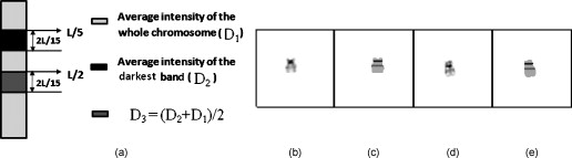

Table 1

Four conditions for potential candidates of chromosome 22.

Number of the DarkestBands (ND)	Darkest Band Index (DI)	Darkest Band Ratio (DR)	Centromere Index (CI)
1	$<0.4$	$>0.02$	$<0.25$

Due to the uncontrollable technical aspects during the clinical processing of the bone marrow specimens, normal chromosomes 22 in different metaphase cells could have variations in the actual length and intensity (pixel value) distribution. Therefore, the length and average intensity of the reference template used in our scheme are adaptively adjusted to fit with different matching candidates. Specifically, in each matching test, the reference template is automatically adjusted to have the same length and the same average intensity as the matching candidate. By computing the length $\left(L\right)$ and average intensity $\left(D_1\right)$ of the matching candidate, we defined the corresponding parameters of the reference template as follows. As shown in Fig. 8, the reference template of chromosome 22 includes two dark bands. However, the intensity levels of these two dark bands are different. The one with higher intensity or pixel value locates around $L∕5$ . The length of this dark band is $2L∕15$ with the average intensity value $\left(D_2\right)$ of the darkest bands in chromosome 22. The second dark band begins at $L∕2$ with the same length as the first dark band $(2L∕15)$ but with a different average intensity level $\left(D_3\right)$ , which is computed by $D_3=(D_2+D_1)∕2$ . Using this adaptively adjusted template, the scheme computes the Pearson’s correlation coefficient $\left({\mathrm{cr}}_1\right)$ between the detected matching candidate and the corresponding template using the following equation:

Eq. 5

$${\mathrm{cr}}_1=\frac{\sum _{i=1}^N(X_i-\overline{X})(Y_i-\overline{Y})}{{\left[\sum _{i=1}^{i=N}{(X_i-\overline{X})}^2\right]}^{1∕2}{\left[\sum _{i=1}^{i=N}{(X_i-\overline{X})}^2\right]}^{1∕2}},$$

where $\overline{X}=\left({\sum }_{i=1}^{i=N}{X}_i\right)∕N$ , $\overline{Y}=\left({\sum }_{i=1}^N{Y}_i\right)∕N$ , $X_i$ is the gray value of $i$ ’ $th$ pixel inside the template, $Y_i$ is the gray value of $i$ ’ $th$ pixel inside the candidate, and $N$ is the total number of pixels within the candidate. The ${\mathrm{cr}}_1$ is defined as the similarity score. By sorting through all the computed similarity scores, the scheme selects one chromosome that has the highest score as the first identified (primary) chromosome 22, which is recorded as 22-1.

After obtaining the primary chromosome 22, there are two methods to detect and identify whether there is the second normal chromosome 22 in a metaphase cell. The first method is to directly select the second candidate in the sorted list of comparing with the reference template as the second chromosome 22. The second method is to use the identified normal chromosome 22 (namely, 22-1) as a new template to redetect whether there is a homologue matching pair for the chromosome 22-1. Although the identified chromosome 22-1 is the most similar to the reference template, there is always a subtle difference between the real chromosome in the metaphase cell and the idealized template. Hence, to further improve detection accuracy, we used the second method to identify the second normal chromosome 22. In this approach, a set of new feature differences are computed and assessed between the identified chromosome 22-1 and each of the remaining candidates. The smaller the feature difference, the higher the degree of similarity is between these two compared chromosomes. Table 2 lists the thresholds of the six feature differences between the chromosome 22-1 and the candidate including (1) the order of the size $\left(R\right)$ , (2) the intensity of a chromosome $\left(I\right)$ , (3) the standard deviation of intensity inside the chromosome (SD), (4) centromere index (CI), (5) the location of darkest band in the chromosome (LD), and (6) the size ratio (SR) between the chromosome 22-1 and the candidate. If the candidate satisfied all six conditions, the scheme further computes the cross-correlation score between the chromosome 22-1 and the candidate. Since the sizes of the potential candidates of chromosome 22 are different, the cross-correlation will be computed within the banding profile instead of the chromosomes themselves. Comparing the length of the potential candidates’ banding profiles with one of the identified primary chromosome 22-1, the shorter length is chosen as a standard to calculate the cross-correlation²⁰ between these two chromosomes. The cross-correlation $\left({\mathrm{cr}}_2\right)$ is computed as

$${\mathrm{cr}}_2=\sum _{i=1}^{i=L}(X_i-\overline{X})(Y_i-\overline{Y})∕\left(S_x{S}_y\right),$$

where $S_x={\left[{\sum }_{i=1}^{i=L}{(X_i-\overline{X})}^2\right]}^{1∕2}$ , $S_y={\left[{\sum }_{i=1}^{i=L_1}{(Y_i-\overline{Y})}^2\right]}^{1∕2}$ , $\overline{X}=\left({\sum }_{i=1}^{i=L}{X}_i\right)∕L$ , $\overline{Y}=\left({\sum }_{i=1}^{i=L}{Y}_i\right)∕L$ , and $L$ is the shorter length between the potential candidate and the identified primary chromosome 22-1. After analyzing all chromosomes in the candidate list and sorting this new set of similarity scores $\left({\mathrm{cr}}_2\right)$ , the scheme selects the one with the highest correlation score among those candidates with ${\mathrm{cr}}_2>0.7$ as the second normal chromosome 22-2. Otherwise, the second normal chromosome 22 is considered not detected (or missing).

Table 2

The similarity score between normal chromosome 22-1 and 22-2.

‖Rr−Rc‖	‖Ir−Ic‖	‖SDr−SDc‖	‖CIr−CIc‖	‖LDr−LDc‖	‖Sr−Sc‖∕Sr
$⩽3$	$<20$	$<30$	$<0.2$	$<0.2$	$<0.3$

Note: r represents the primary chromosome 22-1 and c represents the candidates of 22-2.

3.

Results

Figure 9 displays three examples that show the original microscopic images of the captured metaphase cells and the segmentation and identification results in which most of the individual chromosomes were correctly segmented. After chromosome alignment, the scheme sorts the segmented chromosomes based on their size. Then all separated chromosomes are displayed in the sorted order [Figs. 9, 9, 9]. In the first example [Fig. 9], the cell was obtained from a positive case for CML and the scheme detected only one chromosome 22 [Fig. 9]. In the second and the third examples, the two cells are extracted from two negative cases. The scheme correctly detected and identified two normal chromosomes 22 in both examples. In the second example [Fig. 9], two chromosomes 22 are not overlapped with the other chromosomes in the original metaphase cell. Thus, both chromosomes were correctly segmented without losing any feature information of this specific type of chromosome [Fig. 9]. However, in the third example [Fig. 9], a small fraction of one chromosome 22 was lost during the segmentation process due to the overlapped chromosomes. Hence, this chromosome becomes shorter [Fig. 9]. Despite the loss of partial information, this chromosome was still correctly identified because its cross-correlation score was higher than (1) other candidate chromosomes inside this cell and (2) the predetermined threshold $(>0.7)$ . In addition, although our scheme was unable to correctly segment a few overlapped chromosomes [Figs. 9 and 9], as long as the most fraction of chromosomes 22 were successfully segmented, the segmentation errors did not affect the performance of the scheme to detect suspiciously positive cells or cases for CML.

Fig. 9

Identification results of three metaphase cells including one abnormal cell (a) and two normal cells (c) and (e). In the abnormal cell (a) only one normal chromosome 22 was detected (b) and in two normal cells (c) and (e) two normal chromosomes 22 were detected (d) and (f). (Note: 22-1 is the first identified normal chromosome 22 with the highest similarity score to the reference template and 22-2 is the second identified normal chromosome with the highest similarity score to 22-1.)

Tables 3, 4 summarize the scheme performance in detecting and identifying chromosomes 22 in our testing image data set. In 30 negative cases, the scheme correctly detected and identified the first chromosome 22 (namely, 22-1) in 196 out of 197 cells (including 186 normal cells and 10 abnormal cells). The scheme was unable to detect one normal chromosome 22 in one normal cell. The scheme also detected the second chromosome 22 in 162 out of 187 cells, resulting in missing detecting the second chromosome 22 in 25 cells. Thus, in a total of 384 chromosomes 22 visually identified by the cytogeneticists, the scheme correctly detected 358 of them, resulting in the chromosome-based accuracy rate of 93.2%. For the 197 cells included in the 30 negative cases, 172 were classified as negative cells and 25 were classified as positive cells. Hence, the cell-based accuracy rate is 87.3% (Table 3). In the 30 positive cases, the scheme achieved 94.7% chromosome-based accuracy rate and 94.5% cell-based accuracy rate (Table 4). Combing 30 negative and 30 positive cases together, the chromosome-based and the cell-based accuracy rates are 93.8% $(607∕647)$ and 91.4% $(412∕451)$ , respectively.

Table 3

The results for identifying normal chromosome 22 in 30 negative cases for CML.

Table 4

The results for identifying normal chromosome 22 in 30 positive cases for CML.

The experimental results also show that there are two types of errors resulting in a total of 40 incorrect decisions in the detection and identification of chromosomes 22. The first one is the inability to detect chromosome 22 due to the lower similarity scores (< threshold). The scheme reported that 33 normal chromosomes 22 were missing. The second one is misclassification. In this testing data set, the scheme misclassified one chromosome 19, three chromosomes 20, and three chromosomes 21 as chromosomes 22, respectively. Hence, in this experiment the 82.5% $(33∕40)$ of errors was due to the misdetection and only 17.5% $(7∕40)$ was caused by misclassification. The detailed distribution of these 40 misdetections or misclassifications in both chromosomes 22-1 and 22-2 is shown in Fig. 10 . Since each of 30 positive and 30 negative cases includes multiple analyzable metaphase cells (5 to 20), the scheme detected at least four abnormal cells in each of all 30 positive cases and 4 negative cases (Table 5 ). Based on our preestablished classification rules, the scheme detects 34 positive cases and 26 negative cases in our testing data set. Therefore, the case-based accuracy is 93.3% (56 of 60). The scheme achieved 100% sensitivity and 86.7% specificity when applying to this testing data set.

Fig. 10

Histogram of the misdetection or misclassification of normal chromosomes 22. Note: Error type 1, chromosome 22 is missing (not detected); error type 2, chromosome 19 is misclassified as chromosome 22; error type 3, chromosome 20 is misclassified as chromosome 22; and error type 4, chromosome 21 is misclassified as chromosome 22.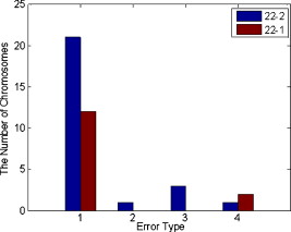

Table 5

The case-based automated classification results.

4.

Discussion

In this study, a new computerized scheme was developed and tested to automatically segment individual chromosomes from the metaphase cells as well as to detect and identify the normal chromosomes of class 22 among the segmented chromosomes. The scheme has a number of unique characteristics. First, we applied and tested a new method to iteratively segment chromosomes with varying gray-level distributions. The experimental results show that this simple iterative thresholding method reduces or minimizes the impact of the large variations in the cell intensity (gray level) on the accuracy and reliability of segmentation. Second, since the chromosomes segmented from the metaphase cell are randomly distributed in both positions and orientations, we applied a series of algorithms to align all segmented chromosome. The experimental results show that these algorithms are able to correctly detect the principal axis of segmented chromosomes in all 24 classes (1-22, X, and Y) and rotate (align) each chromosome into the defaulted orientation, as shown in Fig. 9. Thus, the image features computed from each individual chromosome can be more consistent and comparable in the next step of the template matching. Third, we recognized that chromosomes of the same class in different metaphase cells could be different in both size and intensity distribution due to the uncontrollable clinical environments. To compensate for such variations in the different specimens or cells, we designed a unique dynamic template for chromosome 22. Its parameters (including the length and average intensity level) are adaptively adjusted based on the different matching chromosomes. Fourth, our scheme is a model- or knowledge-based scheme. Unlike the previously reported data-driven template-matching schemes that require training and cross-validation, our approach does not involve any training process (avoiding the issues of possible overtraining). Thus, the entire data set was used to test the scheme performance, which maximizes the capacity of the testing data set and increases the reliability of the testing results.

Our scheme also has a number of unique application characteristics. First, although metaphase chromosome cells can be generated from different specimens (i.e., peripheral blood and bone marrow), the image quality (or visibility) of metaphase cells varies significantly.³⁹ In the diagnosis of leukemia, bone marrow is considered to be the most informative tissue for cytogenetic study. However, karyotyping of metaphase cells obtained from bone marrow is much more difficult due to its lower level of chromosome banding, lower contrast of morphologies, and shorter length. In the clinical practice, the cytogeneticitists typically must spend more time and effort in karyotyping bone marrow compared with peripheral blood or other specimens. Applying computerized schemes for the bone marrow specimens can be potentially more helpful to the clinicians in the clinical practice, but it is also technically more challenging. Therefore, the relatively high accuracy of our scheme when applied to a diverse data set of 451 cells from 60 cases observed in this study is encouraging. The overall cell-based accuracy of 91.4% achieved in this study is very comparable to or higher than the accuracy level reported in previous studies for the similar detection tasks (i.e., 89.1% for detecting normal pair of chromosomes 17 in Ref. 28). Second, although our scheme was only applied to detect and identify chromosome 22, the potential of this scheme is not limited to the detection and classification of this specific chromosome class. Given the existence of the knowledge of all chromosome classes, it would not be difficult to build and test the templates for the other classes of the chromosomes. The image processing steps implemented in our scheme are also relatively easily applied to segment other classes of chromosomes and extract or compute their features with minor modifications.

Despite the encouraging results, this is a preliminary study and it also has a number of limitations. First, the automated separation of severely overlapped chromosomes remains a technical challenge. This is a prime failure of current computerized schemes for automated karyotyping.² However, a computerized scheme that aims to detect and identify only a specific class of chromosomes is less impaired than automated karyotyping. For example, some overlapping chromosomes were not correctly separated in the image, as shown in Fig. 9, but the scheme still correctly detected and identified two chromosomes of class 22. However, since our scheme applies three steps (Fig. 3) to identify chromosome 22, we recognized that similar to all other computerized schemes using multiple processing steps, our scheme can miss a few normal chromosomes of class 22 in any of these three steps. The results of this study also showed that the majority of the error was caused by the misdetection of the chromosomes (82.5%). Thus, improving the performance of automated separation of overlapped chromosomes remains an important research topic in future studies. Second, at the current stage, our scheme can only be used to prescreen for CML based on a simple characteristic of whether the metaphase cell includes two normal chromosomes of class 22. Because the scheme is unable to recognize why the normal chromosomes are not detected, it is not a completely computerized scheme that can actually detect $t(9;22)$ translocation. Third, in our testing data set, the bone marrow specimens are acquired from patients who underwent CML diagnosis and these cases have the $t(9;22)$ translocation involving the distortion of both chromosomes 9 and 22, this scheme only focused on detecting chromosomes 22, which is typically the first chromosome class to be visually detected and analyzed for CML patients in a routine clinical practice. In a future study, we will expand our scheme to detect and identify chromosomes 9, which may help improve the case-based performance in classifying between the positive and negative cases for CML. Finally, we selected a diverse image data set from a clinical database in this study. However, the size of the data set remains relatively small. Therefore, before we can demonstrate any clinical application utility, the performance and robustness of this scheme must be further tested by using much larger and more diverse image data sets in the future studies.