|
|
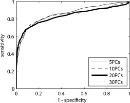
1.IntroductionIn the UK, there are 45,500 newly diagnosed cases of breast cancer and 12,000 deaths every year; in the United States, there are over 200,000 new cases and over 40,000 related deaths per annum.1 Breast cancer spreads first through the lymphatic tracts, to the lymph nodes in the axilla—the region of the armpits.2 Lymphatic spread is a strong indicator of both distant metastases and survival, and their presence informs planning regarding additional treatment after surgery (adjuvant treatment), which includes chemotherapy, hormonal therapy, and radiotherapy. The standard of care has previously been to remove all of the axillary lymph nodes to control local disease and screen for metastases (axillary lymph node dissection, ALND). However, this has associated complications, particularly lymph edema, a painful swelling of the arms with undrained lymphatic fluid. Only 30% of women will typically have lymphatic involvement with cancer, so for around 70% of cases, axillary clearance is unnecessary. Routine ALND changed with the advent of sentinel lymph node biopsy (SLNB), which is accepted as the standard of care in management of patients with early breast cancer.3, 4 Breast cancer will spread in a hierarchical fashion, first involving the sentinel node (the first in the chain) and then the other nodes in the axilla. In some cases, there is more than one chain, so more than one sentinel node. If the sentinel node(s) are free of cancer, ALND is not necessary. If the presence or absence of cancer in a sentinel node can be determined during surgery, then ALND can be completed during the same operation for those who need it. However, conventional histological analysis can take several days to return a result, leaving patients with a period of uncertainty and the possibility of a second admission to the hospital and surgery if cancer is found in a node.5 There is also additional cost involved to the healthcare provider with this approach. Currently, intraoperative diagnosis is carried out using either touch imprint cytology (TIC)6 the microscopic examination of cells obtained by pressing the cut surface of the node onto a glass microscope slide, or frozen section histopathology,7, 8 where the node is snap-frozen and cut within minutes of excision. Both of these techniques require tissue preparation and a skilled, specialized pathologist to be available in real time to provide analysis. Further, the accuracy of these histological and cytological techniques is highly operator-dependent.9 Such a resource is beyond the reach of many UK hospitals and, by extension, hospitals in many parts of the world. This highlights the need for a technique for intraoperative sentinel node analysis that is inexpensive, non-tissue-destructive (to allow subsequent conventional postoperative analysis), rapid, and consistent. Elastic scattering spectroscopy (ESS) is a point-measurement technique10 that has shown early successes in the detection of cancer and precancerous changes.11, 12, 13, 14 Tissue of interest is interrogated with short pulses of white light and the spectrum of the backscattered light analyzed to discriminate between normal and cancer tissue. It is not tissue destructive, requires limited training to use, and has no consumables. Our previous work14 utilized statistical discrimination methods to assign spectra to “malignant” or “nonmalignant” classes, using ESS spectra matched with conventional histology. In this study, we extend this work by creating a “risk map” of an excised sentinel node to provide an automated diagnosis for the node using our optical scanner. If the decision to undertake ALND is to hinge on ESS, it is essential that the false positive rate is minimized to avoid patients undergoing an unnecessary ALND. We optimized our analyses to obtain as high a specificity as possible, 95% being the minimum acceptable, and then chose the approach that gave the highest sensitivity. If cancer in a node is missed during the ESS analysis, this will be detected on subsequent routine histology. Any reasonable ESS sensitivity will hence produce some reduction in second operations. However, the unnecessary axillary clearance instigated by a false positive is irreversible and to be avoided. By reducing our false positive rate, we maximize the population positive predictive value (PPV), which is of most interest in the long-term assessment of this technique. However, in this small data set, maximizing specificity gives a more stable result, and so the question of optimizing PPV will not be discussed further. 2.Materials and Methods2.1.Elastic Scattering SpectroscopyThe ESS system has been described in a number of previous publications.13, 14 In brief, the optical probe used in this study consists of one and one fiber bound closely together in a parallel geometry, resulting in a center-to-center separation, allowing for the fiber cladding. These fibers are brought into perpendicular contact with the tissue to be interrogated. A xenon short arc lamp (Perkin Elmer LS 1130/FX1100, California) delivers short pulses of white light ( , ) via the fiber; the light is collected from the fiber and analyzed using a spectrometer (Ocean Optics S2000). All components are controlled by a laptop computer, which also performs the statistical analysis. The system takes a dark spectrum of the same duration just before the lamp is flashed to compensate for background light. A software-based “autoranging” algorithm is employed to examine the amount of light collected and adjusts the pulse number and integration time to ensure that the CCD does not saturate and that the signal is sufficiently high to give optimal signal-to-noise. Before the collection of clinical data, a spectrum is collected with the fibers held at a short distance from a piece of spectrally flat material (Spectralon, Labsphere, UK). All subsequent spectra are divided by this spectrum to correct for the overall system response. This yields a system-independent measurement reflecting the intrinsic tissue optical properties. 2.2.ESS ScanningRandom point measurements cannot be expected to give an accurate overall picture of lymph nodes—we would expect that a random, noncomprehensive sampling technique would inevitably miss small deposits of tumor in an otherwise healthy node. The smaller the deposit, the less likely random sampling is to coincide with it; and smaller deposits are less likely to be clinically apparent and hence more difficult to deliberately target with the ESS probe. A more comprehensive sampling method was called for and realized in the form of an ESS raster-scanning device. The exposed surface of a typical bivalved node will be uneven, and so a method is required to provide smooth movement of the fiber probe across the sample and simultaneously give good optical coupling between the probe and tissue. We tackled this problem by using a fiber-optic plate (FOP; Hamamatsu Photonics, Japan), illustrated schematically in Fig. 1 . This plate measures by and is thick. It is composed of contiguous optical fibers, running along the short axis. The tissue is pressed firmly but gently against the underside of the plate using a drop of sterile water or saline to ensure good optical coupling where necessary. The point of the optical fiber is coupled to the top surface of the FOP with microscope immersion oil. In this configuration, the image of the tissue is transmitted directly to the fiber via the plate. The numerical aperture of the plate channels is the same as the optical fiber, which means that the ESS geometry is almost perfectly preserved, notwithstanding the small attenuation due to the packing efficiency of the fibers within the plate. Fig. 1Schematic of ESS scanning device (not to scale). The bivalved node is mounted on a mobile scanning stage. It is coupled to a fiber-optic plate above it using a drop of saline or sterile water and gentle but firm pressure. The fiber-optic plate is coupled to a fixed fiber-optic probe with microscope immersion oil. Stepper motors move the scanning stage in an raster pattern to create a grid of spectra at intervals. 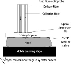 The UV transmission of the FOP is weaker, so to remove any spectral bias introduced by the plate, we performed our system-response calibration with Spectralon through a fiber-optic plate of the same geometry and construction. This flat geometry enabled the smooth and efficient scanning of a area. The node and fiber-optic plate are mounted on an stage driven by stepper motors, and the node and FOP moved together in a raster-scanning pattern relative to the fixed fiber. A step size was used to generate a grid of spectral measurements. Applying the statistical discrimination algorithms allowed the construction of a false color map based on the canonical score for the spectrum from each pixel. 2.3.Study DesignOur standard methodology is based on the statistical discrimination tools described here and requires a data set to train the machine learning algorithms to discriminate between normal and metastatic tissue. Therefore, the study was conducted in two phases: a training phase followed by a validation/test phase. Ethics committee approval was obtained. 2.4.Training DataExcised nodes from patients with a preoperative diagnosis of breast cancer undergoing sentinel node biopsy or ALND were included. Each node was bivalved along its long axis and a set of point ESS spectra collected by placing the optical probe manually on up to 16 random sites on the cut surface. The nodes were then fixed in 10% formalin and sent for routine histopathological analysis with hematoxylin and eosin (H&E) staining. Only nodes that subsequent histology showed to be either completely normal or completely replaced by cancer were used in the training set, avoiding misregistration of the fiber with respect to any metastases in the node. 2.5.Scanned Nodes (Test Set)Patients with a preoperative diagnosis of breast cancer who did not have known cancer in their axillary lymph nodes underwent sentinel lymph node biopsy (SLNB) using the combined technique of blue dye and radiocolloid for node localization.15 In brief, the approximate location of the sentinel node was established by external gamma camera after injection of the colloid into the breast adjacent to the tumor. An incision was then made over this area, and the node was identified by using a handheld gamma detection probe and uptake of blue dye, injected into the breast prior to surgery. Excised nodes were immediately bivalved, ESS scans were taken from the cut surface as described earlier, and the node subsequently fixed in 10% formalin and sent for routine histology. Nodes found to contain cancer on histology were subclassified as macrometastases (cancer deposit ) or micrometastases (cancer deposit ). It is possible to detect smaller cancer deposits using conventional histology or immunohistochemistry. However, the American Society of Surgical Oncology current guidelines do not recommend axillary clearance for metastases , so for the purpose of this study, these nodes have been regarded as nonmetastatic.15 2.6.Algorithm GenerationThe literature on physical correlation of ESS spectra suggests that the spectral components important in ESS are slowly varying, with features on the scale of tens of nanometers.12 Therefore, applying moderate smoothing to ESS data should give improved signal-to-noise without obscuring important features within the spectrum. We applied a halfwidth cubic Savitzky-Golay algorithm. We cropped from , the region in which the signal-to-noise was highest, and reduced the data set by taking every seventh point. This reduced the size of each spectrum from 1000 to 87 points, ameliorating the computational complexity of the statistical analyses to follow. Analysis of the training data set was undertaken by extracting spectral features using principal component analysis (PCA)16 and discriminating between classes by linear discriminant analysis (LDA).17 By projecting the spectral vector onto the axis of maximum discrimination, we derive a canonical score, which is our predictive measure of cancer risk. The resulting discrimination algorithms could then be applied to unseen spectra in the second phase of the study. The per-spectrum accuracy of the algorithm was assessed by leave-one-out cross-validation. These analyses were carried out in the statistical programming language R,18 and a number of algorithms developed for 5, 10, 15, 20, and 30 principal components (PCs). The optimum is chosen with reference to the scanned nodes, as described later. It should be noted that these PCs will contain the majority of the variation within the data set. 2.7.Image AnalysisIn the previous section, the statistical procedure for analyzing individual spectra was described; we then developed tools to analyze the map of canonical scores and produce a binary decision of whether the node contained cancer, and hence whether an axillary clearance was called for. It is desirable in the operating theater that interpretation of these images by the surgeon or a pathologist is not required, and that an automated and operator-independent result is generated by the system. The training data provides a rule (or more precisely, a number of rules, depending on the number of principal components selected and the cut-off applied to the canonical score) for classifying a pixel, but this needs to be extended to a rule for classifying an image. Making a diagnosis of a whole node based on isolated spectra is not reliable enough, with a considerable overlap between the canonical scores of spectra from normal and metastatic areas giving rise to individual false-positive pixels. In a tumor area, however, we are more likely to see a “clump” of positive pixels, so we considered that the simplest approach would be a “clump-counting” method. A clump was defined as a series of positive pixels contiguous via their vertical or horizontal but not diagonal edges. Diagonal contiguity was not considered because the distance between pixel centers linked diagonally is , compared to the for the horizontal/vertical separations. The volume of tissue interrogated at each position of the fiber probe is addressed in the following discussion. We examined all of the clumps within a node and counted the number of pixels within each clump. The size of the largest clump within the node was used for the classification of the whole node. This was implemented by an iterative counting method; each metastatic pixel was identified in turn. Any metastatic neighboring pixels were noted; in the next cycle, any metastatic neighbors of these pixels were noted; and so on, iteratively, until no more contiguous neighbors were found. This gave rise to a clump size associated with every metastatic pixel; in general, these will not be unique—e.g., if all of the metastatic pixels in a hypothetical node are found in one clump of size 10, this analysis will generate 10 clump sizes, each of them having numerical value 10. Because we use only the largest clump size, this redundancy does not compromise our results. The most robust test of discrimination accuracy would be achieved by using a test set independent of the data sets used to train the PCA/LDA algorithm and tune the additional discrimination parameters. For this study, there was a limited data set available, and so it was necessary to choose a statistical method that offered as robust an approach as possible, while acknowledging that a completely prospective test is not sensible. In order to both tune the classification rule and get a realistic assessment of its likely performance, the following leave-one-out procedure was adopted, with two variants: leave-one-node-out (LONO) and leave-one-patient-out (LOPO). The second approach should remove any overfitting due to the patients with multiple nodes: 40% of the patients had two or more sentinel nodes scanned, and 10% had three or more nodes scanned. Leaving out one node, or one patient, the classification rule was tuned on the remaining data. Three parameters were varied: the number of principal components used for the algorithm (5, 10, 15, 20, 30); the canonical score cut-off (0.5, 1.0, 1.5, 2.0, 2.5); and the clump size (1–20: In theory, we could allow this to vary from 0 to 400, but we want to ensure that the smaller metastases are not excluded. corresponds to metastases in diameter). The tuning criterion was to find the highest sensitivity for a specificity of 95% or greater. The resulting tuned rule, and only this rule, was then used to classify the omitted node or nodes. This was repeated, leaving out each node, or patient, in turn. The result of this exercise is a classification for each node in which the tuning has been done without using the node being classified. One implication of the procedure is that the tuned rule may be different every time, and thus any assessment of performance using the resulting classifications does genuinely incorporate the uncertainty in the tuning process. Comparing the leave-one-out predictions with the known histology for the nodes, we generated four headline figures: sensitivity, specificity, (population) positive predictive value (PPV), and (population) negative predictive value (NPV). These are referred to as the leave-one-out results. The rules generated for each left-out node/patient were compared to investigate the stability of the tuning process, and the modal rule was identified and applied to all the nodes to generate a further set of predictions. We refer to the latter as the modal result. 3.Results3.1.Training SetThe training set used in the first phase to develop the diagnostic algorithm consisted of 2989 spectra (2722 normal and 267 metastatic) collected from 361 nodes (330 completely normal and 31 completely metastatic) excised from 205 patients (184 with completely normal nodes and 21 with at least one completely metastatic node). The leave-one-out analysis of our initial training set yielded a canonical score for each spectrum. Figure 2 shows the distribution of canonical scores for the 20-PC algorithm; the normal nodes have an asymmetric peak with a mean of and a standard deviation of 0.8. In contrast, the metastatic scores are widely distributed between and (mean 2.4, standard deviation 2.4), with no clear structure within that range. It seems that the algorithm has the ability to classify the normal tissue consistently while giving a range of scores for the metastatic tissue. This is typical for the algorithms generated using other numbers of PCs (not shown). Fig. 2Distribution of canonical scores generated from the point-measurement training set. We show the scores generated using an LDA from 20 PCs.  By varying the cut-off, a receiver operator characteristic (ROC) curve for per-spectrum discrimination was generated for the point-measurement training set (Fig. 3 ). These gave similar results irrespective of the number of PCs used, with an area under curve (AUC) of 0.83 to 0.85 and sensitivities of 0.68 to 0.70 for a specificity of 0.90. It should be remembered that these results were generated on “totally normal” and “totally metastatic” nodes only; in these polarized cases, we might expect the gross changes to be detectable, no matter the number of PCs considered. However, the scanned nodes contained subtler cases—potentially, tumors as small as —and there is no guarantee that each algorithm would be as sensitive in detecting these smaller deposits of cancer. We therefore selected a range of PCs (5, 10, 15, 20, and 30) and generated algorithms for each, to be validated in the next stage. 3.2.Scanned NodesThe scanned set comprised 129 nodes from 81 patients, including 72 normal, 3 with submicrometastases (regarded as nonmetastatic for this study), 4 containing micrometastases, and 50 with macrometastases. This constitutes 1 node each from 49 patients, 2 nodes each from 24 patients, 3 nodes each from 4 patients, 4 nodes from 1 patient, 5 nodes each from 2 patients, and 6 nodes from 1 patient. Figures 4 and 5 show examples of scanned nodes with corresponding photographs. Applying the discrimination rules in a leave-one-out fashion gave us an estimate of the best combination of parameters and their accuracies. In optimizing specificity, the optimal parameters for both leave-one-node-out (LONO) and leave-one-patient-out (LOPO) analyses were 20 PCs, a canonical score cut-off of 2.0, and a clump size of . This choice of parameters was identical for all runs in the LOPO and LONO analyses. The LONO and LOPO analyses both gave a leave-one-out specificity of 96% and a sensitivity of 69%, which was (trivially) identical to the modal result. Assuming a population prevalence of 30% and the same sensitivities and specificities, this choice of parameters would give us a positive predictive value (PPV) of 88% and a negative predictive value (NPV) of 88%. When considering macrometastases only, the sensitivity rises to 71%. Fig. 4A sample scanned node containing metastatic deposits. (a) The false-color map was constructed using point-wise analyses of spectra by a 20-PC LDA algorithm. Red shows regions of metastases; blue normal tissue. (b) Binary map on a cutoff of 2.0—pink identifies cancer; black normal tissue. (c) Photograph of cut surface of node. The two regions show (1) normal tissue and (2) a central region of normal tissue surrounded by a halo of metastases. 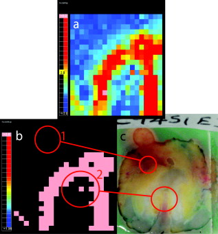 Fig. 5Sample scanned node showing a metastatic deposit (confirmed on histology). (a) Scanned false-color image using 20 PCs. (b) Binary map based on a cutoff of 2.0—pink identifies regions of cancer; black denotes normal tissue or background. (c) Photograph of cut surface of node. This deposit was not detected with touch imprint cytology—possibly because the metastatis was below the cut surface of the node. However, this is an isolated case, and one should not draw too many conclusions from it.  Each pixel is separated by , so a tumor with circular cross section that is detected in only gives a diameter of at least ; we do not want to introduce criteria that make us any less sensitive, indeed we would like greater sensitivity (see Sec. 4). We examined different parameter sets with an eye to improving PPV and found that it was very difficult to obtain a PPV above 90% in the leave-one-out analysis, possibly due to the small numbers involved in this data set—and therefore chose to focus on the sensitivity and specificity. 4.DiscussionIn normal clinical practice, the surgeon will identify and excise the sentinel lymph node at the beginning of the breast cancer operation. It will then typically take for a surgeon to perform a mastectomy or a wide local excision (“lumpectomy”), and this is the window of opportunity for intraoperative lymph node diagnosis. The prototype scanner took to scan of the surface of single node, comparable to the time required for TIC, and certainly well within the required time scale. If we compare the ESS results drawn from the whole data set to the TIC results in the literature,6, 9 we see that while TIC has very robust specificity (typically, 98 to 99%), the sensitivity varies enormously depending on operator, from 100% to as low as 23% (Ref. 9). This source quotes a typical sensitivity of 63%, to which ESS compares favorably. In the literature,6 TIC has 75% sensitivity to macrometastases compared to the ESS result of 71%. However, TIC is much less sensitive to micrometastases; within this data set, ESS detected two of four micrometastases. The numbers are too small for the difference to be statistically significant, but this result is encouraging. We do not expect either technique to be sensitive to the presence of isolated tumor cells, but the American Society of Clinical Oncology states that this is not essential for optimum clinical practice. Frozen section histology is the main alternative to touch imprint cytology, is employed in centers in other parts of the world, and achieves 67 to 75% sensivity and 100% specificity,7, 8 dependent on whether the cancer is lobular or ductal. Clearly, ESS needs to be able to compete with these techniques if it is to be of interest to clinicians. Early indications are encouraging, but it will be necessary to examine a larger data set before this can be assessed fully. Sentinel node analysis techniques such as the rapid polymerase chain reaction, a gene assay, are sensitive enough to detect isolated tumor cells and are potentially more sensitive even than immunohistochemistry staining.19 The disadvantages of this technique are that it currently has large capital costs and expensive consumables and is tissue destructive. Furthermore, it is not clear that this degree of sensitivity is required in this application, when even the clinical significance of micrometastases is not fully agreed upon. The simple, non-tissue-destructive and potentially inexpensive ESS method may be more appropriate and would likely be within the reach of more centers around the world. In the long term, it will be essential to assess the smallest metastases that ESS is able to detect. To be comprehensive, the technique would have to be able to detect metastases as small as (the definition of micrometastases). Small tumor deposits in lymph nodes have an aspect ratio close to unity; it is unusual to see “fingers” of invasive tumor at this scale. For simplicity, let us consider a tumor covering and having circular cross section, detected in all of the pixels of a grid. If we treat the measurement extent of ESS as small compared to the step size, metastases with a radius of less than , the distance between pixels on the diagonals, will not be sufficient to declare a node as positive for cancer. However, this is not a constraint imposed by the ESS geometry, but rather the image analysis rules. It would be desirable in the future to detect micrometastases, and in doing so, it would be necessary to detect cancer in a single pixel. It is here that the ESS sampling volume becomes important. Sample volume is a complex issue with regards to ESS. The mean path that light takes and degree of variation about this path are highly sensitive to the absorption and scattering properties of the tissue. We carried out Monte Carlo simulations based on existing code20 at some typical tissue values to examine the maximum scattering depths for our geometry. Figure 6 plots these voxel visualizations for 3000 collected photons from a material with optical properties representative of tissue at (highly scattering, highly absorbing, , ) and (where absorption is substantially lower but scattering still significant: , ). For each photon, we record the maximum depth of a scattering event (MDSE), which determines how deeply that photon will have traveled into the tissue. This parameter can be averaged over all photon paths, weighted by the final photon intensity to account for the attenuation incurred by the longer path lengths. The MDSE values place an upper limit on the depths probed by the geometry. Fig. 6Monte Carlo simulation of photon transport for a homogeneous tissue-like material. Photons were injected at , and collected at , ; these plots show binned voxel visualisations of scattering events. (a) , (reasonable values for tissue at , where absorption is highest). (b) , (reasonable values for tissue at , where absorption is lower).  For , , the mean MDSE is , the modal MDSE is , the standard deviation of the MDSE is , and 90% of photon contributions have an MDSE of less than . For , , the mean MDSE is , the modal MDSE is , the MDSE standard variation is , and 90% of photon contributions have an MDSE of less than . In both cases, the sample volume extends in the direction; therefore, we might expect any tumor that substantially occupies these volumes to be readily detectable at any wavelength sensitive to metastatic change. The modal MDSE values suggest that a tumor with diameter lying close to the cut surface will occupy the detection volume and be identified by ESS, but this neglects the effects of the presence of tumor on photon path, which is not well understood. Smaller deposits may be detectable, but this is a complex question beyond the scope of this article and will require further investigation of the interaction of tumor properties, scatter sampling volume, energy deposition/absorption volumes, and their relative contribution to the ESS signal. 5.Future WorkBased on these approximations, we see that the criterion puts a lower limit on detectable tumors of over in diameter. If ESS is sensitive to micrometastases, we do not want to limit its efficacy by our image analysis rules; future work will aim to increase ESS sensitivity while retaining specificity. Scanning smaller steps, repeating scans, and repeating measurements at each step will have overlapping advantages—namely, of repetition and resolution. Repetition will average out noise and allow the removal of outlier data that might give false-positive or false-negative pixels. An increase in resolution will increase sampling in the plane and potential sensitivity; and increasing the resolution further to create overlapping measurements will allow further checks of spectrum-to-spectrum consistency and spatial correlation. With the current prototype scanner, it takes to scan the cut surface of the node and generate the false color map. The majority of this time is due to the raster-scanning motion; a smaller portion to spectra collection; and a tiny minority (typically ) due to spectral processing, discrimination, and image generation. The next-generation scanner is able to scan the same area in , and we hope to reduce this time further by simple improvements in the spectrometer. Recent work within our group has utilized statistical analysis of repeated measurements to remove clinical variability in ESS spectra taken in Barrett’s esophagus21; although we are not prey to the same sources of noise, an analogous method might be employed for removing spectral noise and other sources of variation. Another potential methodology is to create a “coarse scan” at the current resolution and then scan a region of interest (i.e., a region containing positive pixels) at a higher resolution. Other workers have succeeded in creating simple and transparent analytical models to describe ESS spectra in terms of basic tissue optical properties.20, 22, 23 Our statistical analysis makes no assumptions about the underlying tissue changes that occur when lymph nodes become cancerous but leaves us without a scientific understanding of the physical and biological structures. The standard-normal-variate normalization that we utilize by necessity redistributes information in different parts of the spectrum. For example, regions with zero “loadings” do not have zero contribution to the analysis—because the spectral data from these regions is used in the normalizations, and hence implicitly in the final analysis. Furthermore, no region of the spectrum is clearly dominant in these loadings. Physical analysis will be a key goal of future work if we want to understand the underlying physiological changes and generalize analyses from lymph node to other organs. However, we will need to ensure that the correct calibrations and supporting data, such as spectra from standard phantoms, are collected at the time of the measurement, which will require a new data set. Prospective prediction and comparison with histological gold standards will be the litmus test for our machine-based approaches, and further clinical study will be key in demonstrating the accuracy and robustness of our approach to sentinel lymph node biopsy. 6.ConclusionsWe have demonstrated an operator-independent optical method for immediate automatic detection of metastatic sentinel lymph nodes based on a scanning ESS system. The headline figures of 69% sensitivity and 96% specificity are close to the standard intraoperative cytological techniques. The technique is fast enough to be applied intraoperatively, is non-tissue-destructive, does not require the presence or expertise of a specialized pathologist, is potentially inexpensive, and requires no consumables and minimal training. Future work will explore physical correlation, while in parallel ensuring the comprehensive scanning of the node. To demonstrate and further assess the effectiveness of the current technique, we want to carry out a multicenter prospective clinical study on a larger number of patients. AcknowledgmentsWe gratefully acknowledge research funding from the U.S Department of Defense Breast Imaging Program (Award No. W81XWH-04-1-0589) and from Hamamatsu Photonics, Hamamatsu, Japan. We are further pleased to acknowledge that this work developed in part as an extension to our participation in the National Institutes of Health (NIH) Network on Translational Research on Optical Imaging (NTROI) program (U54 CA104677). This work was undertaken at UCLH/UCL, who received a proportion of funding from the Department of Health’s NIHR Biomedical Research Centers funding scheme. The views expressed in this publication are those of the authors and not necessarily those of the Department of Health. This work was supported by the Experimental Cancer Medicine Centre, University College London. ReferencesA. Jemal, T. Murray, E. Ward, A. Samuels, R. C. Tiwari, A. Ghafoor, E. J. Feuer, and M. J. Thun,
“Cancer statistics, 2005,”
Ca-Cancer J. Clin., 55 10
–30
(2005). https://doi.org/10.3322/canjclin.55.1.10 0007-9235 Google Scholar
U. Veronesi, G. Paganelli, G. Viale, A. Luini, S. Zurrida, V. Galimberti, M. Intra, P. Veronesi, C. Robertson, P. Maisonneuve, G. Renne, C. D. Cicco, F. D. Lucia, and R. Gennari,
“A randomized comparison of sentinel-node biopsy with routine axillary dissection in breast cancer,”
N. Engl. J. Med., 349 546
–553
(2003). https://doi.org/10.1056/NEJMoa012782 0028-4793 Google Scholar
P. J. Tanis, O. E. Nieweg, R. A. V. Olmos, E. J. T. Rutgers, and B. B. Kroon,
“History of sentinel node and validation of the technique,”
Breast Cancer Res., 3 109
–112
(2001). https://doi.org/10.1186/bcr281 Google Scholar
M. R. S. Keshtgar and P. J. Ell,
“Clinical role of sentinel-lymph-node biopsy in breast cancer,”
Lancet Oncol., 3
(2), 105
–110
(2002). https://doi.org/10.1016/S1470-2045(02)00652-6 1470-2045 Google Scholar
D. Chicken, N. Sivanadarajah, and M. Keshtgar,
“Patients’ view on intraoperative diagnosis of sentinel nodes in breast cancer: is it an automatic choice?,”
Int. J. Surg., 5
(2), 76
–80
(2007). https://doi.org/10.1016/j.ijsu.2006.01.009 Google Scholar
E. Barranger, M. Antoine, D. Grahek, P. Callard, and S. Uzan,
“Intraoperative imprint cytology of sentinel nodes in breast cancer,”
J. Surg. Oncol., 86
(3), 128
–133
(2004). https://doi.org/10.1002/jso.20067 0022-4790 Google Scholar
S. van de Vrande, J. Meijer, A. Rijnders, and J. H. Klinkenbijl,
“The value of intraoperative frozen section examination of sentinel lymph nodes in breast cancer,”
Eur. J. Surg. Oncol., 35
(3), 276
–280
(2009). 0748-7983 Google Scholar
J. W. Horvath, G. E. Barnett, R. E. Jimenez, D. C. Young, and S. P. Povoski,
“Comparison of intraoperative frozen section analysis for sentinel lymph node biopsy during breast cancer surgery for invasive lobular carcinoma and invasive ductal carcinoma,”
World J. Surg. Oncol., 24
(7), 34
(2009). https://doi.org/10.1186/1477-7819-7-34 Google Scholar
K. Tew, L. Irwig, A. Matthews, P. Crowe, and P. Macaskill,
“Meta-analysis of sentinel node imprint cytology in breast cancer,”
Br. J. Surg., 92
(9), 1068
–1080
(2005). https://doi.org/10.1002/bjs.5139 0007-1323 Google Scholar
I. Bigio and J. Mourant,
“Ultraviolet and visible spectroscopies for tissue diagnostics: fluorescence spectroscopy and elastic-scattering spectroscopy,”
Phys. Med. Biol., 42
(5), 803
–814
(1997). https://doi.org/10.1088/0031-9155/42/5/005 0031-9155 Google Scholar
T. Upile, W. Jerjes, C. Betz, M. El Maaytah, A. Wright, and C. Hopper,
“Optical diagnostic techniques in the head and neck,”
Dent. Update, 34
(7), 410
–412, 415–416, 419–420
(2007). 0305-5000 Google Scholar
A. Sharwani, W. Jerjes, V. Salih, B. Swinson, I. Bigio, M. El-Maaytah, and C. Hopper,
“Assessment of oral premalignancy using elastic scattering spectroscopy,”
Oral Oncol., 42
(4), 343
–349
(2006). https://doi.org/10.1016/j.oraloncology.2005.08.008 0964-1955 Google Scholar
L. B. Lovat, K. Johnson, G. D. Mackenzie, B. R. Clark, M. R. Novelli, S. Davies, M. O’Donovan, C. Selvasekar, S. M. Thorpe, D. Pickard, R. Fitzgerald, T. Fearn, I. Bigio, and S. G. Bown,
“Elastic scattering spectroscopy accurately detects high grade dysplasia and cancer in Barrett’s oesophagus,”
Gut, 55
(8), 1078
–1083
(2006). https://doi.org/10.1136/gut.2005.081497 0017-5749 Google Scholar
K. Johnson, D. Chicken, D. Pickard, A. Lee, G. Briggs, M. Falzon, I. Bigio, M. Keshtgar, and S. Bown,
“Elastic scattering spectroscopy for intraoperative determination of sentinel lymph node status in the breast,”
J. Biomed. Opt., 9
(6), 1122
–1128
(2004). https://doi.org/10.1117/1.1802191 1083-3668 Google Scholar
G. H. Lyman, A. E. Giuliano, M. R. Somerfield, A. B. Benson III, D. C. Bodurka, H. J. Burstein, A. J. Cochran, H. S. Cody III, S. B. Edge, S. Galper, J. A. Hayman, T. Y. Kim, C. L. Perkins, D. A. Podoloff, V. H. Sivasubramaniam, R. R. Turner, R. Wahl, D. L. Weaver, A. C. Wolff, and E. P. Winer,
“American Society of Clinical Oncology guideline recommendations for sentinel lymph node biopsy in early-stage breast cancer,”
J. Clin. Oncol., 23
(30), 7703
–7720
(2005). https://doi.org/10.1200/JCO.2005.08.001 0732-183X Google Scholar
K. Pearson,
“On lines and planes of closest fit to systems of points in space,”
Philos. Mag., 2
(6), 559
–572
(1901). 0031-8086 Google Scholar
R. Fisher,
“The use of multiple measurements in taxonomic problems,”
Ann. Eugen., 7 179
–188
(1936). Google Scholar
M. Martin Martinez, I. Veys, S. Majjaj, L. Lespagnard, J. Schobbens, G. Rouas, V. Filippov, D. Noterman, D. Hertens, F. Feoli, P. Bourgeois, V. Durbecq, D. Larsimont, and J. Nogaret,
“Clinical validation of a molecular assay for intra-operative detection of metastases in breast sentinel lymph nodes,”
Eur. J. Surg. Oncol., 35
(4), 387
–392
(2009). 0748-7983 Google Scholar
G. Zonios, L. T. Perelman, V. Backman, R. Manoharan, M. Fitzmaurice, J. Van Dam, and M. S. Feld,
“Diffuse reflectance spectroscopy of human adenomatous colon polyps in vivo,”
Appl. Opt., 38
(31), 6628
–6637
(1999). https://doi.org/10.1364/AO.38.006628 0003-6935 Google Scholar
Y. Zhu, T. Fearn, G. Mackenzie, B. Clark, J. M. Dunn, I. J. Bigio, S. G. Bown, and L. B. Lovat,
“Elastic scattering spectroscopy for detection of cancer risk in Barrett’s esophagus: experimental and clinical validation of error removal by orthogonal subtraction for increasing accuracy,”
J. Biomed. Opt., 14
(4), 044022
(2009). https://doi.org/10.1117/1.3194291 1083-3668 Google Scholar
A. Amelink, J. Haringsma, and H. Sterenborg,
“Noninvasive measurement of oxygen saturation of the microvascular blood in Barrett’s dysplasia by use of optical spectroscopy,”
Gastrointest. Endosc., 70
(1), 1
–6
(2009). https://doi.org/10.1016/j.gie.2008.08.039 0016-5107 Google Scholar
R. Reif, O. A’Amar, and I. J. Bigio,
“Analytical model of light reflectance for extraction of the optical properties in small volumes of turbid media,”
Appl. Opt., 46
(29), 7317
–7328
(2007). https://doi.org/10.1364/AO.46.007317 0003-6935 Google Scholar
|