3.1.

Time-Gated FLIM

To implement time-gated FLIM, we employed a novel time-domain, wide-field FLIM system for picosecond time-resolved imaging for biological applications [Fig. 1].^{5, 23} A dye laser (GL-301, Photon Technology International, Lawrenceville, New Jersey) pumped by a nitrogen laser (GL-3300, Photon Technology International, Lawrenceville, New Jersey) for UV–visible–near-infrared (NIR) excitation provided a wide-field, less expensive, and potentially portable alternative to multiphoton excitation for subnanosecond FLIM of biological specimens.²³ A sample was illuminated by an excitation pulse, and the fluorescence emission was recorded by an intensified charge-coupled device (ICCD) camera (Picostar HR, LaVision, Germany) at a gate delay controlled by the intensifier, with emission intensities integrated during a gate width. The ICCD had variable intensifier gain and gate width settings varying from $200\mathrm{ps}\text{to}10\mathrm{ms}$ and could be used to implement high-speed imaging in other applications as well.²⁴ In addition, this system had a large temporal dynamic range ( $750\mathrm{ps}$ to ∞), $50\mathrm{ps}$ lifetime discrimination, and spatial resolution of $1.4\mu \mathrm{m}$ , which made it very suitable for studying a variety of endogenous and exogenous fluorophores in biological samples.^{2, 4, 25, 26, 27, 28} Fluorescence lifetime maps were determined by first acquiring fluorescence intensity images at four delays and then calculating the lifetime values from the intensity images on a pixel-by-pixel basis (described in Sec. 3.2).

The gating parameters [the gate width, $g$ , and the time interval between the starting points of two consecutive gates, $dt$ , see Fig. 1] can be optimized by using MC simulations^{10, 11, 12} or applying error propagation (described in Sec. 3.4).

3.2.

Four-Gate Lifetime Mapping

To create fluorescence lifetime maps rapidly, a four-gate protocol with a linearized least-squares lifetime determination method was used on a pixel-by-pixel basis. This method is more precise than the two-gate protocol while still easy to implement,^{11, 29, 30}

Additional steps in data processing are needed for more accurate lifetime map production. Before lifetime calculation, the step “background subtraction” takes average of the intensities of pixels within a specified background region and subtracts that average value from all pixels. After background subtraction, the step “reject” sets intensities to zero for all pixels with intensities below a certain value (assigned as the parameter “reject”). After lifetime calculation, the step “ $\tau$ range” sets lifetimes to zero for all pixels with lifetimes above a certain value (assigned as the parameter “taurange”) to remove lifetime values in physically meaningless regions. In this study, “reject” was set to 10 and “taurange” was set to 15.

3.3.

Sample Preparation and Imaging

Fluorescent beads with diameters of $10\mu \mathrm{m}$ (Cat. no. 18140, Polysciences, Warrington, Pennsylvania) were suspended in distilled water to produce a solution with a final concentration of $1.5\times {10}^6\text{beads}∕\mathrm{mL}$ . Before imaging, $200\mu \mathrm{L}$ of the solution was placed on a $\delta$ T dish (Bioptechs, Butler, Pennsylvania), and the imaging process with the time-gated FLIM system was begun after the beads had settled to the bottom of the dish. All beads had excitation/emission maxima of $441∕486\mathrm{nm}$ , as specified by the manufacturer. A 40× microscope objective was used. The voltage across the microchannel plate of the intensifier was set at $800\mathrm{V}$ . The beads were excited at ${\lambda }_{\mathrm{ex}}=436\pm 10\mathrm{nm}$ using the laser dye coumarin 440 and the fluorescence was collected at ${\lambda }_{\mathrm{em}}=480\pm 20\mathrm{nm}$ .

3.4.

Optimal Gating

In this study, single-exponential gating optimization was utilized. The optimal gating of the four-gate protocol [Eq. 4] was first determined by MC simulations, in which the relative standard deviation (RSD) (defined as the standard deviation divided by the mean value) of the determined lifetime values was minimized by changing the gate width $\left(g\right)$ and the time interval between the starting points of two consecutive gates $\left(dt\right)$ , assuming that only Poisson noise was present (Fig. 2 ). In addition, $g$ and $dt$ did not vary with different gates, meaning that once $g$ and $dt$ are chosen for a simulation, the $g$ values for all the four gates are the same and the $dt$ values between the first and second, second and third, and third and fourth gates are the same as well. For a different simulation, new $g$ and $dt$ values will be chosen. Because these distributions were constructed by MC simulations with the repetitive addition of noise, RSD provided a quantitative measurement of the precision of the determination of a certain parameter, such as lifetime. Because this study considered only a single-exponential decay, the intensity profile could be written as $I\left(t\right)=\alpha \exp (-t∕\tau )$ , and the RSD of either $\alpha$ (the pre-exponential term) or $\tau$ (the lifetime) could be minimized. In this study, we optimized the gating scheme for the best precision of $\tau$ determination.

Fig. 2

MC simulation procedure for evaluating the precision of lifetime determination. The decay model $I\left(t\right)$ , gate width $g$ , time interval $dt$ between two consecutive gates, and the correct values of lifetime $\tau$ and pre-exponential term $\alpha$ were used to simulate the noise-free integrated fluorescence intensity. Then, Poisson noise was added, and the $\tau$ and $\alpha$ values retrieved from the noise-corrupted signals (denoted as ${\tau }^{\prime }$ and ${\alpha }^{\prime }$ ) were recorded in each iteration to build up a histogram over a number of iterations of noise addition and lifetime determination. The RSD was calculated from the histogram distribution, and this histogram buildup process was then repeated with different $g$ and $dt$ values. The optimal $g$ and $dt$ occurred when minimal RSD values were achieved. In this study, single-exponential decay was considered and RSD was evaluated only for $\tau$ .

Alternatively, the RSD of the lifetime determined by the four-gate protocol could be analytically determined by applying error propagation to Eq. 4, with the assumption that the variance of the fluorescence intensity was the same as the intensity magnitude, which is a characteristic of Poisson noise. Again, the optimal gating parameters were determined when the minimal RSD was achieved.

As mentioned above, other forms of noise in addition to Poisson noise may appear in real imaging systems. This will be considered in our future studies and should further improve FLIM precision with optimal gating.

3.5.

Total Variation Denoising

Two approaches were used with TV denoising to improve the precision of lifetime determination in FLIM. In “lifetime denoising” [Fig. 3 ], a lifetime map was first constructed by four-gate lifetime mapping. Because the variance of lifetime was not proportional to the lifetime values, VWTV [Eq. 2] was used. The variance estimation, as a function of $\tau$ , $g$ , $dt$ , and total photon counts [(TC), the photon counts integrated under the entire decay curve, see Fig. 1], was performed by analytically solving the error propagation of Eq. 4, which led to the following equation:

Fig. 3

The precision of lifetime determination in FLIM was improved by either (a) lifetime denoising, where the estimated variance of lifetime values was used in VWTV for denoising of lifetime maps or (b) intensity denoising, where estimated $G$ was used in FWTV for denoising of each intensity image before four-gate lifetime mapping.

4.1.

Determining Optimal Gating

The RSD values as a function of lifetime-scaled $dt$ and $g$ were consistent (Fig. 4 ) whether obtained from the MC simulation (Fig. 2) or the analytical solution [derived from Eq. 4], especially for high total photon counts (or $\mathrm{TC}=\mathrm{10,000}$ ). The analytical solution suggests that the RSD of lifetime is inversely proportional to ${\left(\mathrm{TC}\right)}^{1∕2}$ , which can be observed in Figs. 4 and 4: The contours had exactly the same shapes with tenfold differences in their values. When TC was large enough $(\mathrm{TC}=\mathrm{10,000})$ , the MC simulation and analytical results were consistent. When TC was small $(\mathrm{TC}=100)$ , higher RSD values were predicted by MC simulation in the outer nonoptimal regions.

Fig. 4

Contour plots of the relative standard deviation (RSD) of the lifetime values determined by MC simulation (Fig. 2) with (a) $\mathrm{TC}=\mathrm{10,000}$ , (b) $\mathrm{TC}=100$ and by analytical solution [derived from Eq. 4] with (c) $\mathrm{TC}=\mathrm{10,000}$ and (d) $\mathrm{TC}=100$ . $dt$ and $g$ were scaled by the lifetime $\tau$ . The analytical solution suggests that the RSD of lifetime is inversely proportional to ${\left(\mathrm{TC}\right)}^{1∕2}$ , which can be observed in (c) and (d). When TC was large enough $(\mathrm{TC}=\mathrm{10,000})$ , the MC simulation and analytical results were consistent. When TC was small $(\mathrm{TC}=100)$ , higher RSD was predicted by MC simulation in the outer nonoptimal regions. The dashed lines $(g∕\tau =3)$ were further inspected with $dt∕\tau =0.15$ , 0.3, 0.75, and 1.5 (labeled with open circles) in Fig. 5 along with experimental data. Number of MC $\text{simulations}=\mathrm{10,000}$ . The sampling grids: For MC simulation, $dt∕\tau =0.05–1.5$ with 0.05 increments and $g∕\tau =1–10$ with 0.5 increments; for analytical solution $dt∕\tau =0.05–1.5$ with 0.01 increments and $g∕\tau =1–10$ with 0.1 increments.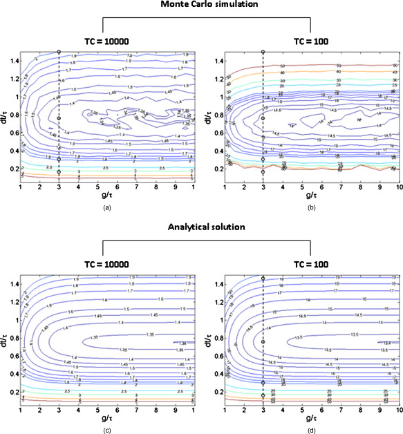

Fig. 5

Percent RSD (relative standard deviation) in calculated lifetime (dashed lines and open circles in Fig. 4) and experimentally measured lifetime, as a function of the time interval $dt$ (in nanoseconds) between two consecutive gates. The RSD values of the measured lifetime were determined from the lifetime values retrieved from the nonzero pixels in the FLIM images of the experimentally prepared fluorescent beads. The simulation/analytically determined value of optimal $dt$ $\left(2.5\mathrm{ns}\right)$ was verified by the experiments to produce lower lifetime RSD than the surrounding $dt$ values. The gate width was fixed at $10\mathrm{ns}$ , and the TC were 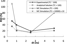$\sim 100$ .

Indeed, we do not expect the results from both methods to be exactly the same. The accuracy of the analytical solution may suffer from the linearization approximation in error propagation derivation, therefore underestimating the RSD when the errors were highly nonlinear at low photon counts [Fig. 4 versus Fig. 4]. On the other hand, the MC simulation should be more accurate at low photon counts, but the accuracy may suffer from the limited number of simulations and the usually more discretized parameter values used as inputs for the simulations.

In spite of the differences in the results of the two methods, both results from the MC simulations and the analytical solutions suggested the same optimal gating scheme, which was independent of TC: The optimal $dt$ was $\sim 0.75$ of the lifetime value and the optimal $g$ should be greater than at least threefold of the lifetime value (only negligible improvement exists once $g⩾4\tau$ ). In this case, the gates actually overlap. Although the determination of the optimal gating scheme requires the lifetime value of the sample, an approximate lifetime value is usually available from previous knowledge of the sample, or a test experiment with arbitrary gating.

Therefore, for the fluorescent bead sample mentioned above (Sec. 3.3) with lifetime value of $\sim 3.3\mathrm{ns}$ (determined with the time-gated FLIM system), the optimal gating should be around $dt=2.5\mathrm{ns}$ and $g⩾10\mathrm{ns}$ . This prediction was validated experimentally, as shown in Fig. 5 .

What can also be observed in Fig. 4 is that apparently RSD had a greater dependence on $dt$ than on $g$ . Therefore, in our experimental validation of the optimal gating (Fig. 5), we only changed $dt$ (the open circles in Fig. 4) around its optimal value, $2.5\mathrm{ns}$ , while having $g$ fixed at $10\mathrm{ns}$ (the dashed lines in Fig. 4).

Figure 5 shows that the RSD curve from analytical solution $(\mathrm{TC}=100)$ overlapped with that from MC simulation $(\mathrm{TC}=\mathrm{10,000})$ multiplied by 10. This means that when TC was high, the curves from two approaches were consistent. As mentioned previously, the MC simulation at low TC predicted higher RSD when the gating was not optimal. All these three curves had the minimal RSD at $dt=2.5$ ns, which was confirmed by the RSD curve from the experimental data.

The above approach assumed single-exponential decay. If the number of components in the sample is unknown, then the suggested procedure will be to use the optimal gating of single-exponential decay first, aiming at the averaged lifetime value, to acquire the least noisy overall decay behavior. This curve can then be fitted with single- and double-exponential decay to determine which one fits the curve better. For a decay curve with more than two components, however, more than four gates will be needed (see below).

As for the optimal gating with more than one decay component, first, we can further apply the optimal gating schemes of double-exponential decays, which have been constructed in our laboratory, for lifetime precision improvement, either independently or in combination with image denoising.¹⁴ More than two components can also be considered in the future, using the same procedure shown in Fig. 2. However, in this case, at least $2\times \left(\text{the}\text{number}\text{of}\text{decay}\text{components}\right)$ gates are needed to fit the intensity profile and solve all the parameters (there are one lifetime and one pre-exponential term for each component), and the computational work for the optimal gating determination will become much more complicated.

4.2.

Improving Precision of Lifetime Determination in Time-Gated FLIM

4.2.1.

Reduction in relative standard deviation

Optimal gating, lifetime denoising, and intensity denoising all improve FLIM precision. This is demonstrated in Fig. 6 , where the noise distribution within the FLIM maps of fluorescent beads is illustrated. We note that this is a fairly low-light case with total photon counts only around 100. The holes inside the fluorescent beads [Fig. 6] came from one of the lifetime calculation steps, in which the $\tau$ values above a certain threshold were set to zero. Because this threshold was set to $\tau =15\mathrm{ns}$ , random fluctuations in low-light imaging caused some pixels to have lifetime values more than four times larger than the expected values if the gating scheme was not optimal. After intensity denoising [Fig. 6], the image became smoother and the RSD value dropped to 46%, but the extremely high $\tau$ values above the threshold still could not be removed. This was similar to the lifetime-denoised map [ $\mathrm{RSD}=49\mathrm{\%}$ , Fig. 6]. Optimal gating [Fig. 6] removed these artifacts and further decreased the RSD value to 20.1%, as well as reducing the diameter of the beads so that it became closer to the actual bead size of $10\mu \mathrm{m}$ . This effect on the spatial pattern was actually due to the fact that more pixels were properly “rejected” in data processing (Sec. 3.2) after denoising. Further improvement was then achieved by denoising the optimally gated image with either the denoising approach [ $\mathrm{RSD}=14.7\mathrm{\%}$ and 13.7%, Figs. 6 and 6, for lifetime denoising and intensity denoising, respectively]. A comparison of Fig. 6 to Fig. 6 [or to Fig. 6] shows that most of the remaining lifetime random variations within the beads in the optimally gated image could be removed by denoising. Here, the combination of optimal gating and TV denoising resulted in about a fourfold improvement in precision. In addition, the results in Fig. 6 suggested that the improvement from the intensity denoising ( $\sim 6\mathrm{\%}$ , in this case) could be independent of that from optimal gating ( $\sim 32\mathrm{\%}$ , in this case). Although 6% may seem small relative to an RSD of 51.5% (nonoptimal gating), it is quite large relative to an RSD of 20.1% (optimal gating), because it is a one-third reduction in RSD. Therefore, image denoising is particularly important when optimal gating is also applied.

Fig. 6

FLIM images of fluorescent beads acquired with a gate width of $10\mathrm{ns}$ and different values of the time interval $dt$ between two consecutive gates: (a) $dt=0.5\mathrm{ns}$ , undenoised; (b) $dt=2.5\mathrm{ns}$ (optimal), undenoised; (c) $dt=0.5\mathrm{ns}$ , lifetime denoised; and (d) $dt=2.5\mathrm{ns}$ (optimal), lifetime denoised; (e) $dt=0.5\mathrm{ns}$ , intensity denoised; and (f) $dt=2.5\mathrm{ns}$ (optimal), intensity denoised. The nonoptimally gated intensity images, optimally gated intensity images, and their corresponding FWTV-denoised images are shown in Fig. 7. The improvements in precision by optimal gating and TV denoising in combination are easily observable in this low-light case $(\mathrm{TC}=\sim 100)$ . The labeled RSD values were obtained from all pixels with lifetime of $>2$ to remove the variations from the background values. Scale bar: $10\mu \mathrm{m}$ .

Fig. 7

The (a) nonoptimal and (b) optimal gating schemes, and (c) the nonoptimally and (d) optimally gated intensity images, and (e,f) their corresponding FWTV-denoised images, respectively, used to obtain the results shown in Fig. 6. In (a) and (b), the red solid lines represent gate start time points, while the blue dotted lines represent corresponding gate end time points in the same sequence from left to right. (c–f) are shown in the same spatial order as the intensity image stacks representing them in Fig. 6. Also, in each of (c–f), gates 1–4 are shown in the upper-left, upper-right, lower-left, and lower-right panels, respectively. Scale bar: $10\mu \mathrm{m}$ . (Color online only.)

The nonoptimally and optimally gated intensity images, their gating schemes, and their corresponding FWTV-denoised images are shown in Fig. 7 . We can clearly see that, because the optimal gating had a larger $dt$ value [Fig. 7 versus 7], the intensity decay trace could be more easily observed in Fig. 7 compared to Fig. 7. This was also true for Fig. 7 compared to Fig. 7. On the other hand, after denoising, the removal of noise [Fig. 7 versus Fig. 7 and Fig. 7 versus Fig. 7] was obvious while the geometry of the beads was not affected.

In this section, we conclude that optimal gating and image TV denoising can be employed either independently or in combination to improve precision in low-light time-gated FLIM. When these two methods are combined, their overall fourfold (from 51.5 to 13.7%) improvements in precision can be easily observed in our low-light example (Fig. 6).

4.3.

Broader Applications

Our techniques can be further applied to time-correlated single-photon counting (TCSPC) FLIM, which is a commonly used method for live-cell lifetime imaging. Optimal gating could be applied to TCSPC FLIM by virtual gating, in which the values of data points within each virtual gate were summed up to form an intensity image. The four-gate protocol can again be used for virtually gated TCSPC FLIM. Similarly, denoising approaches, including both intensity denoising and lifetime denoising, can also be applied to TCSPC FLIM. It has been demonstrated that a greater than fivefold improvement in lifetime precision can be achieved in TCSPC FLIM images when optimal virtual gating and TV denoising are applied in combination.³¹

As for the image denoising methods alone, it will be interesting and useful to employ, optimize, and compare other image denoising techniques specifically for the applications of FLIM, either independently or in combination with optimal (virtual) gating.

Finally, because optimal denoising improves other advanced image processing techniques such as image deconvolution,³² segmentation, and object tracking, the combination of denoising and these techniques can also be studied specifically for FLIM use.