2.1.

Data Collection and Calibration

A two-channel Periflux 5000 (Perimed AB, Järfälla, Sweden) modified for $50\text{-}\mathrm{kHz}$ digital recording of the detected signals (time varying part—ac; static light intensity—dc) was used for data collection. The wavelength of the light source (diode laser) was $780\mathrm{nm}$ . The probe was custom built by Perimed AB, with one light-emitting fiber placed in the center, one light-collecting fiber placed $0.25\mathrm{mm}$ (center-to-center distance) from the light-emitting fiber, and another 11 light-collecting fibers placed in a circle $1.2\pm 0.1\mathrm{mm}$ from the light-emitting fiber. All fibers were made of silica with a $0.125\text{-}\mathrm{mm}$ diameter and $\mathrm{NA}=0.37$ .

The recorded Doppler power spectra were noise-compensated by subtracting noise spectra compiled from static measurements at corresponding dc levels. The spectra were then ${\mathrm{dc}}^2$ -normalized to make them independent of the average light intensity. Additional compensation for the spectral characteristics of the system was also performed.¹⁰ Unlike conventional LDF, the latter step is important, especially at low frequencies below about $100\mathrm{Hz}$ .

In conventional LDF, the perfusion signal is calibrated using a measurement in a motility standard of a certain size distribution, concentration, and temperature. In order to be able to compare the measured and simulated spectra, another calibration procedure has been used in this study. The measured spectra were normalized by the total power of a spectrum from a measurement in motility standard (in principle, any scattering liquid would be appropriate), where all photons have been Doppler shifted due to Brownian motion with frequency shifts within the signal bandwidth. Thus, the total power for frequencies above $0\mathrm{Hz}$ in the normalized spectra corresponded to the level of Doppler-shifted photons, and could thus be compared to simulated or forward-calculated spectra in an absolute manner. It should be noted that the calibration measurement had to be averaged over a relatively long time interval, about $30\mathrm{s}$ , in order to cancel out high-power, low-frequency fluctuations in the calibration spectra.

2.2.

Skin Model

The basic idea of the proposed method is to iteratively adjust an optical skin model until its output data matches measured LDF data. The model used is a three-layered structure consisting of one epidermal layer and two dermal layers. This is a simplification and generalization of a previously presented six-layered model.¹⁰ The epidermal layer has a variable thickness and contains no blood, whereas the dermal layers contain variable amounts of blood of variable speed distribution (Sec. 2.3.3). The superior dermal layer is $0.5\mathrm{mm}$ thick, and the second dermal layer has an infinite thickness. The optical properties of epidermis and dermis at $780\mathrm{nm}$ are given in Table 1 . (Ref. 10) Note that the refractive index $n$ is set to 1.40 to avoid Fresnel reflections at the distinct borders between the layers.

Table 1

Optical properties of bloodless skin at 780nm .

The blood in the model was assumed to have 80% hemoglobin oxygenation, 43% hematocrit, a hemoglobin value of $145\mathrm{g}$ Hb/liter blood, and mean cell hemoglobin concentration (MCHC) of $345\mathrm{g}$ Hb/liter RBC. Given those values, the absorption coefficient of blood at $780\mathrm{nm}$ is $0.43{\mathrm{mm}}^{-1}$ (Ref. 11). The scattering coefficient ${\mu }_{\mathrm{s}}$ was set to $222{\mathrm{mm}}^{-1}$ , and the phase function was set to a Gegenbauer kernel phase function with ${\alpha }_{\mathrm{Gk}}=1.0$ and $g_{\mathrm{Gk}}=0.948$ , resulting in an anisotropy factor $g$ of 0.991 and a reduced scattering coefficient ${\mu }_{\mathrm{s}}^{\prime }={\mu }_{\mathrm{s}}(1-g)=2.0{\mathrm{mm}}^{-1}$ (Ref. 10).

2.3.

Forward Problem

In the forward problem, the Doppler power spectrum for a given RBC tissue fraction, speed distribution, and epidermal thickness is calculated. The forward problem is based on Monte Carlo simulations, but as these are time consuming, a fast post-processing technique is proposed that allows for an approximate, yet accurate, solution to the forward problem. For calculating the Doppler power spectrum using this post-processing technique, knowledge is needed about the intensity of backscattered photons from each layer and the path-length that the photons have propagated in each layer. That knowledge is used for calculating the distribution of the number of Doppler shifts that the photons have accumulated in each layer. For all layers, these distributions are combined with single-shifted optical Doppler spectra, calculated using the assumed speed distribution, to produce a simulated Doppler power spectrum. The first part of the proposed method for post-processing photon transport in a multilayered structure not only is limited to LDF simulations but could also be used for studying tissue absorption effects. The following subsections describe the proposed method in detail. A flowchart giving an overview of the forward problem is shown in Fig. 1 .

Fig. 1

Flowchart showing the forward problem of calculating a Doppler power spectrum from a given set of skin model parameters.

2.3.2.

Doppler power spectrum

For calculating the Doppler power spectrum, the shift distribution, i.e., the distribution of the number of Doppler shifts each photon undergoes, is needed. This can be calculated for each layer using the normalized modified path-length distribution $p_{\mathrm{pl},m,n}^{″}\left(d\right)=p_{\mathrm{pl},m,n}^{\prime }\left(d\right)∕{\sum }_j{p}_{\mathrm{pl},m,n}^{\prime }\left(d_j\right)$ , the blood tissue fraction in the layer ${\zeta }_{\text{blood},m}$ , and the scattering coefficient of blood, ${\mu }_{\mathrm{s},\text{blood}}$ :

Eq. 5

$$p_{\text{Shifts},m,n}\left(s\right)=\sum _{j=1}^D{p}_{\mathrm{pl},m,n}^{″}\left(d_j\right)\mathrm{Po}(s,\mu ),$$

where $\mathrm{Po}(s,\mu )$ denotes the probability of obtaining $s$ number shifts from a Poisson distribution with parameter $\mu =d_j{\zeta }_{\text{blood},m}{\mu }_{\mathrm{s},\text{blood}}$ (Ref. 12).

For a known speed distribution in each layer, a single-shifted optical Doppler spectrum $G_1\left(\beta \right)$ can be generated with knowledge on the scattering phase function of the RBCs, assuming an isotropic relationship between the direction of the photon and the direction of the RBCs. In $G_1\left(\beta \right)$ , $\beta$ denotes the frequency. This spectrum is calculated as a histogram from $2.5\text{million}$ Doppler-shifted photons, where each Doppler shift $f_{\mathrm{D}}$ is stochastically generated using

Eq. 6

$$f_{\mathrm{D}}=-\mathbf{v}\cdot \mathbf{q}=-2\frac{v}{\lambda }\sin \frac{\theta }{2}\cos \phi ,$$

where $v=\left|\mathbf{v}\right|$ is the speed of the RBCs; $\mathbf{q}$ is the difference between the wave vectors ${\mathbf{k}}_{\mathrm{i}}$ and ${\mathbf{k}}_{\mathrm{s}}$ of the incident and scattered light wave, respectively; $\lambda$ is the wavelength in the medium; $\theta$ is the scattering angle; and $\phi$ is the angle between $\mathbf{q}$ and $\mathbf{v}$ . In this stochastic generation of Doppler shifts, $v$ is randomly chosen from the speed distribution (see Sec. 2.3.3), $\theta$ is randomly chosen from the scattering phase function of the RBCs, and $\cos \phi$ is randomly chosen from a uniform distribution between $-1$ and 1.

The optical Doppler spectrum for any $s$ number of shifts can be calculated using the cross-correlation:

Eq. 7

$$G_s\left(\beta \right)=G_{s-1}\left(\beta \right)\star G_1\left(\beta \right)$$

$G_0\left(\beta \right)$ , i.e., the non-Doppler-shifted spectrum, equals the Dirac delta function. Since $G_s\left(\beta \right)$ can be assumed to be symmetric around $\beta =0$ (equal amount of positive and negative Doppler shifts), the cross-correlation can be replaced by a convolution. By Fourier transforming $\left(\mathcal{F}\{\dots \}\right)$ the optical Doppler spectrum, we can thus write:

Eq. 8

$$Y\left(\gamma \right)\equiv \mathcal{F}\left\{G_1\left(\beta \right)\right\}\Rightarrow \mathcal{F}\left\{G_s\left(\beta \right)\right\}=Y^s\left(\gamma \right).$$

We now extend the notation to $Y_{m,n}\left(\gamma \right)$ , where $m$ and $n$ are used in analogy with Eq. 2. The Fourier transformed multiple Doppler-shifted spectrum for all photons in layer $m$ that have been propagating down to layer $n$ can then be calculated as

Eq. 9

$$Y_{\mathrm{ms},m,n}\left(\gamma \right)=\sum _{s=0}^S{p}_{\text{Shifts},m,n}\left(s\right)Y_{m,n}^s\left(\gamma \right).$$

The next step is to summarize the spectra from all layers by cross-correlating them, i.e., calculating the product in the Fourier domain:

Eq. 10

$$Y_{\mathrm{ml}}\left(\gamma \right)=\sum _{n=1}^N{I}_n^{\prime }\prod _{m=1}^n{Y}_{\mathrm{ms},m,n}\left(\gamma \right),$$

where $I_n^{\prime }=I_n∕{\sum }_m{I}_m$ . Last, the Doppler power spectrum is calculated as

Eq. 11

$$P_{\mathrm{D}}\left(f\right)={\mathcal{F}}^{-1}\left\{Y_{\mathrm{ml}}^2\left(\gamma \right)\right\},$$

where the square is introduced because the Doppler power spectrum equals the autocorrelation of the optical Doppler spectrum¹³.

An example of the forward calculation is given in Fig. 2 , where the light thin spectra originate from calculations of the three-layered model, and the dark thick spectra originate from a conventional Monte Carlo simulation of the same setup, i.e., based on the cumulative Doppler shift of each detected photon. The conventional Monte Carlo simulation lasted for several hours, while the forward calculation took on the order of one millisecond per spectrum using an ordinary PC and utilizing its graphics card for hyper-parallel computation.

Fig. 2

Example of the forward-calculated spectra at two different source–detector separations ( $0.25\mathrm{mm}$ lower, $1.2\mathrm{mm}$ upper) from a three-layered model (light thinline), compared to Monte Carlo simulated spectra of the same setup (jagged blackline). The spectral difference was calculated to ${\chi }^2=0.12$ (see Sec. 2.4.2).

2.3.3.

Speed distribution

The speed distribution in each layer is controlled by two parameters that control the slopes, i.e., the derivative, of the distribution for low and high speeds, respectively, in the loglog plane. Furthermore, the slope for speeds below $0.1\mathrm{mm}∕\mathrm{s}$ is zero, and the slope at $200\mathrm{mm}∕\mathrm{s}$ is $-50$ . The transition between the various slopes is smooth. An example showing the speed distribution with slopes of $-2$ and $-1$ for low and high speeds, respectively, is shown in Fig. 3 . The slopes for the low and high speeds are also drawn in that figure, as well as the zero slope for speeds below $0.1\mathrm{mm}∕\mathrm{s}$ and the slope of $-50$ at $200\mathrm{mm}∕\mathrm{s}$ . Those four slopes and smooth transitions between them constitute the speed distribution.

Fig. 3

Illustration of the speed distribution used; the thin lines indicate the slope or derivative at various speeds.

2.4.

Inverse problem

To find the optimal skin model for a given measurement, the nonlinear inverse problem of matching calculated spectra to the measured spectra is solved using the Levenberg-Marquardt method. In each iteration, the forward problem is solved for the two source–detector separations 0.25 and $1.2\mathrm{mm}$ using the same skin model parameters. The resulting calculated Doppler power spectra are then compared to the corresponding measured Doppler power spectra. Global convergence of the algorithm is ensured by using multiple start positions. Solving the inverse problem from a starting point relatively close to the solution (for example, the solution in the most recent measurement) takes about $0.5\mathrm{s}$ with our implementation of the method using the graphics card on an ordinary desktop computer. A flowchart giving an overview of the inverse problem is shown in Fig. 4 .

Fig. 4

Flowchart showing how the inverse problem is solved ensuring global convergence.

2.5.

Derived quantities

The estimated quantities in qLDF are given from the optimal best-fit model. The presented quantities are given for a half-sphere placed immediately beneath the light-emitting fiber of the probe, with a volume of $3{\mathrm{mm}}^3$ (radius $1.13\mathrm{mm}$ ); see Fig. 5 . This volume is called the output volume, and the quantities from the three layers are weighted depending on the relative part of the half-sphere that each layer occupies. The RBC tissue fraction, average RBC speed, and perfusion (the RBC tissue fraction times their average speed), are given for three speed intervals: below $1\mathrm{mm}∕\mathrm{s}$ , $1$ to $10\mathrm{mm}∕\mathrm{s}$ , and above $10\mathrm{mm}∕\mathrm{s}$ . The RBC tissue fractions and perfusions in these intervals are simply summarized to give the total RBC tissue fraction and perfusion, respectively, and the mean total speed is calculated by dividing the perfusion with the RBC tissue fraction. Furthermore, the RBC tissue fraction is given in the unit $\mathrm{g}\mathrm{RBC}∕100\mathrm{g}$ tissue, the speed in mm/s, and the perfusion in $\mathrm{g}\mathrm{RBC}∕100\mathrm{g}$ $\text{tissue}\times \mathrm{mm}∕\mathrm{s}$ . The RBC tissue fraction is given from the blood tissue fraction of the model, where the blood was set to a hematocrit level of 43%, hemoglobin value of $145\mathrm{g}$ Hb/liter blood, and MCHC of $345\mathrm{g}$ Hb/liter RBC. A tissue density of $1.04\mathrm{kg}∕\text{liter}$ is assumed.¹⁵

Fig. 5

Illustration of the output volume (half-sphere). The derived quantities are calculated from the model properties within this volume. The banana shapes represent the main probed volumes for the short $(\rho =0.25)$ and long $(\rho =1.2)$ source–detector separations. The emitting fiber is labeled $e$ .

3.1.

Three-Layered Models

The qLDF method was evaluated using simulations of three-layered models that could be exactly mimicked by the qLDF model itself. In total, six different setups with various epidermal thicknesses, blood tissue fractions, and speed distributions were evaluated. One extreme case of the three-layered model is when the epidermal layer thickness is zero and the two dermal layers are identical—i.e., a homogeneous model. Such a model constituted one of the six models.

The deviation between the estimated and true perfusion in these six models was between $-9.2\mathrm{\%}$ and 3.4% for the total perfusion. For the separate perfusion in the three speed regions, the deviation was between $-8.1\mathrm{\%}$ and 7.7% relative to the total perfusion. For all six models, the perfusion in the lowest speed region was slightly underestimated, 3.8% on average and maximum 5.2%, whereas the perfusion in the highest speed was overestimated, 4.5% on average and maximum 7.7%.

3.2.

Random Models

For a more objective robustness analysis, the method was also tested on random setups of a complex seven-layered skin model. The top layer of that model mimicked an epidermal layer with variable thickness. Below the epidermis, six dermal layers were located, with variable thicknesses, blood tissue fractions, and speed distributions of the type described in Sec. 2.3.3. The thickness of the epidermal layer and the first five dermal layers was randomly chosen between 0 and $0.3\mathrm{mm}$ , whereas the last dermal layer extended to an infinite depth. For each setup, the blood tissue fraction, mean speed, and perfusion (blood tissue fraction times mean speed), were not allowed to differ more than a factor of 50 between the six dermal layers.

For comparison, both the qLDF and the cLDF method were evaluated on 50 of these random models. For the cLDF method, the perfusion was estimated separately at the two source–detector separations by calculating the first moment of the Doppler power spectra.

The total true perfusion of the simulated model, sorted in ascending order, is plotted against the estimated perfusion in Fig. 6 , and against the conventional perfusion estimates for the two source–detector separations in Fig. 6. The conventional perfusion estimates are normalized to attain a median of the 10 lowest points that equals the median of the true perfusion. For these 10 values, the perfusion is assumed to be in the linear region. The median of the absolute (i.e., ignoring the sign) relative difference between the true and estimated perfusion was 12% using the quantitative method. The corresponding difference for the normalized conventional perfusion estimates was 25% for the short source–detector separation and 26% for the long one. It can be noted that the conventional perfusion estimate, especially for the long source–detector separation, becomes rather nonlinear at high perfusion levels, due to multiple Doppler shifts. Apart from this nonlinearity, the perfusion estimate for the long separation shows a higher robustness (low level of fluctuations) than for the short separation.

Fig. 6

True total perfusion (thick line, dots) from the 50 simulated random models versus the estimated perfusion using the new method [(a), crosses] and versus the conventional perfusion estimates (b) at source–detector separations $0.25\mathrm{mm}$ (crosses) and $1.2\mathrm{mm}$ (plus signs).

The median difference between the perfusion estimates and the true perfusion for the three individual speed regions did not exceed 6% for any of the speed intervals, relative to the total true perfusion. The relative difference for the total estimated perfusion was between $-40$ and 61%, $-14$ and 74% for speeds below $1\mathrm{mm}∕\mathrm{s}$ , $-16$ and 21% in the interval $1$ to $10\mathrm{mm}∕\mathrm{s}$ , and $-34$ and 41% for speeds above $10\mathrm{mm}∕\mathrm{s}$ . The median relative difference between the estimated and true perfusions relative to the total perfusion for the lowest speed region was 2%, for the middle speed region $-3\mathrm{\%}$ , for the highest speed region $-3\mathrm{\%}$ , and for the total perfusion $-5\mathrm{\%}$ .

3.3.

Optical Properties of Static Media

The models presented in this and the coming sections (i.e., Secs. 3.3, 3.4, 3.5, 3.6) are based on the six-layered skin model presented in Ref. 10. Unlike that model, the speed distribution was smooth, as described in Sec. 2.3.3. For the standard six-layered skin model, the deviation between the total estimated perfusion and true perfusion was 0.0%, with $-6.7\mathrm{\%}$ for the lowest speed region, $-1.1\mathrm{\%}$ for the middle speed region, and 7.8% for the highest speed region.

The sensitivity to variations in absorption coefficient of the epidermal layer was evaluated in four different setups. This coefficient is foremost dependent on the tissue fraction of eumelanin. The evaluated absorption coefficients of 0.1, 0.4, 1.6, and $7.7{\mathrm{mm}}^{-1}$ correspond to a melanin tissue fraction of 0, 2, 10, and 50%, which can be compared to fractions of about 1 to 3% for fair skin and up to about 43% for black skin.^{16, 17}

The absorption coefficient of dermis as well as the scattering coefficient for both epidermis and dermis was also evaluated. These optical properties were varied between $-2$ and 2 standard errors from the mean values presented in Ref. 18, corresponding to $18.7$ to $27.3{\mathrm{mm}}^{-1}$ for ${\mu }_{\mathrm{s}}$ in epidermis, $0.064$ to $0.136{\mathrm{mm}}^{-1}$ for ${\mu }_{\mathrm{a}}$ in dermis, and $10.4$ to $15.6{\mathrm{mm}}^{-1}$ for ${\mu }_{\mathrm{s}}$ in dermis. The effect of changing these optical properties, including the eumelanin tissue fraction, was negligible except for the absorption coefficient of dermis. The findings are summarized in Table 2 , where the relative deviations between the estimated and true perfusion are given, both for the total perfusion and for the perfusion in the three different speed regions relative to the total true perfusion.

Table 2

Relative deviation (%) between the estimated and true perfusions when changing the optical properties of epidermis and dermis.

3.4.

Optical Properties of Blood

A change in the hemoglobin oxygen saturation will change the absorption coefficient of blood. Totally reduced hemoglobin increases the absorption coefficient from $0.43$ to $0.58{\mathrm{mm}}^{-1}$ $(+35\mathrm{\%})$ , whereas totally oxygenized hemoglobin decreases it from $0.43$ to $0.39{\mathrm{mm}}^{-1}$ $(-9\mathrm{\%})$ . Furthermore, the absorption coefficient of blood is directly proportional to the mean cell hemoglobin concentration (MCHC) and the hematocrit. Therefore, the effect of a changed ( $\pm 40\mathrm{\%}$ , $0.26$ to $0.6{\mathrm{mm}}^{-1}$ ) absorption coefficient of blood was evaluated. In analogy, the effect of a changed ( $\pm 40\mathrm{\%}$ , $133$ to $311{\mathrm{mm}}^{-1}$ ) scattering coefficient of blood was evaluated.

The RBC shape and formation (aggregation) have an impact on the scattering phase function.¹⁹ The effect of this has been evaluated by varying the anisotropy factor $g$ of the scattering phase function of the RBCs from the standard value of 0.991. As the Doppler shift is dependent on $1-g$ rather than on $g$ , $1-g$ was varied $\pm 40\mathrm{\%}$ , resulting in $g$ from 0.9874 to 0.9946. For the applied Gegenbauer kernel phase function using ${\alpha }_{\mathrm{Gk}}=1.0,$ this interval corresponds to a $g_{\mathrm{Gk}}$ between 0.9365 and 0.9610.

The effect on the perfusion estimate when changing the absorption coefficient of blood is negligible. The situation is the contrary when changing the scattering properties of blood. This is summarized in Table 3 .

Table 3

Relative deviations (%) between the estimated and true perfusions when changing the optical properties of blood.

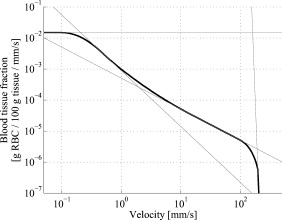
3.5.

Discrete Blood Vessels

For the three-layered model used in the presented method, the blood is homogeneously distributed in the layers. The effect of this simplification was also evaluated by simulating models containing discrete blood vessels. The speed distribution in these blood vessels was parabolic, with zero speed at the vessel wall and twice the average speed in the center.

The effect of locating most of the low-speed flow into discrete capillaries was negligible (within 5% for the total perfusion as well as for the perfusion in the different flow speed regions), even when the capillaries were located directly beneath the source or detector fiber. This was true when the capillaries were placed both in parallel with the skin surface or perpendicular to the skin surface. In these simulations, capillaries with an inner diameter of $8\mu \mathrm{m}$ were distributed with a density corresponding to approximately 20 capillary loops per ${\mathrm{mm}}^2$ .

For larger blood vessels, on the other hand, the result is very much dependent on the exact location of the vessels. When a large vessel is located just outside the $3\text{-}{\mathrm{mm}}^3$ half-sphere volume, it does not affect the true perfusion within the volume, but it still affects the Doppler power spectra and thus the estimated perfusion. In such a situation, the estimated perfusion will be overestimated. However, when a relatively large vessel is located deep in the $3\text{-}{\mathrm{mm}}^3$ volume, the perfusion is instead underestimated, but when it is placed shallowly just below the emitting fiber, it is again overestimated, since the Doppler power spectra are largely affected by the vessel. To test this, simulations were performed where a $50\text{-}\mu \mathrm{m}$ vessel with mean speed of $3\mathrm{mm}∕\mathrm{s}$ (parabolic flow profile) was successively moved downward in the six-layered skin model, between 0.15 and $1.7\mathrm{mm}$ below the surface. The vessel was placed in parallel with the skin surface and directly beneath both the light-emitting fiber and the light-collecting fiber at $0.25\mathrm{mm}$ . In Fig. 7 , the true and estimated total perfusion are plotted as a function of vessel depth, whereas the relative difference between the estimated and true total perfusion is plotted in Fig. 7, together with the ${\chi }^2$ -error between the simulated Doppler power spectra and the Doppler power spectra calculated from the best-fit model. Two examples of the spectral fit (depths 0.5 and $1.1\mathrm{mm}$ ) are shown in Fig. 8 .

Fig. 7

Estimated (squares) and true (circles) perfusion are plotted in (a), and the relative difference between them (circles) and the ${\chi }^2$ -error of the model fit (squares) in (b), as a function of the depth of the $50\text{-}\mu \mathrm{m}$ vessel. The outer radius of the output volume $\left(1.13\mathrm{mm}\right)$ is marked on the depth scale.

Fig. 8

Spectral fit between simulation (jagged blackline) and adapted model (smooth lightline) when the $50\text{-}\mu \mathrm{m}$ vessel is located at the depth $0.5\mathrm{mm}$ [(a), ${\chi }^2=1.6$ ] and $1.1\mathrm{mm}$ [(b), ${\chi }^2=0.22$ ].

3.6.

Hair and Sweat Glands

The effect of a hair and a sweat gland in the skin was evaluated. The root of the hair shaft was placed straight below the illuminating fiber, in the center of the reticular dermis. It was modeled as a $0.4\text{-}\mathrm{mm}$ -long cylinder, with a diameter of $170\mu \mathrm{m}$ , tilting away from the closest detector fiber.²⁰ The hair shaft was modeled as a $0.7\text{-}\mathrm{mm}$ -long cylinder, with a diameter of $40\mu \mathrm{m}$ , that extended the hair root and penetrated the epidermis surface about $0.3\mathrm{mm}$ away from the illuminating fiber. The optical properties of the hair were approximated to ${\mu }_{\mathrm{a}}=2.0{\mathrm{mm}}^{-1}$ , ${\mu }_{\mathrm{s}}=13{\mathrm{mm}}^{-1}$ , $g=0.85,$ and $n=1.55$ .

The sweat gland was modeled as a $20\text{-}\mu \mathrm{m}$ -diam, $0.1\text{-}\mathrm{mm}$ cylinder placed between the illuminating fiber and the closest light-collecting fiber, perpendicular to the tissue surface. The optical properties of the sweat gland were set to ${\mu }_{\mathrm{a}}=0{\mathrm{mm}}^{-1}$ , ${\mu }_{\mathrm{s}}=2{\mathrm{mm}}^{-1}$ , $g=0.85,$ and $n=1.33$ . The refractive index is equal to the refractive index of water, which is most likely an underestimation.

The results showed a negligible effect for both the hair and the sweat gland, within 5% for both the total perfusion and for the perfusions in the different flow speed regions.

5.1.

Methodological Considerations

The presented qLDF measures are separated into three speed regions; below $1\mathrm{mm}∕\mathrm{s}$ , $1$ to $10\mathrm{mm}∕\mathrm{s}$ , and above $10\mathrm{mm}∕\mathrm{s}$ . These measures are given for a half-sphere with a volume of $3{\mathrm{mm}}^3$ . Additional volumes of 1, 2, 4, and $5{\mathrm{mm}}^3$ were also tested. However, since the $3\text{-}{\mathrm{mm}}^3$ volume gave the smallest deviations for the random models presented in Sec. 3.2, and also for the six-layered skin model, that volume was chosen. This volume covers almost equal parts of the two dermis layers of the three-layered model (depending on the epidermal thickness) and is between the measurement volumes normally probed in skin at $780\mathrm{nm}$ using the 0.25- and $1.2\text{-}\mathrm{mm}$ source–detector separations.⁵ The volume is arbitrary and could be chosen without any distinct borders to better represent the probed volume, and that volume could be dependent on the best-fit model. This would increase the robustness of the method but would also significantly obstruct the physiological interpretation of the results, as the output volume would be nonconstant. The choice of speed regions is arbitrary. However, due to the number of free model parameters and their effect on the speed distribution of the model, it does not seem reasonable to have more than three regions.

In addition to the presented three-layered model with six free model parameters, the performance of a number of other models was also evaluated. The previously presented six-layered skin model¹⁰ with various number of free parameters and speed components was evaluated, as well as two-layered models and other variants of the three-layered model. However, the current model was chosen due to its high degree of generality—i.e., its ability to adjust to different microcirculatory conditions—and its robustness.

The ${\chi }^2$ -error is used for selecting the best model, but can also be used as an estimator of the reliability of the perfusion estimate. A large ${\chi }^2$ -error suggests that the three-layered model could not adapt to the measured spectra, and the estimated perfusion measures are then not reliable. This can be seen for example in Fig. 8, where ${\chi }^2=1.6$ and the deviation of the estimated total perfusion to the true perfusion is $-43\mathrm{\%}$ . We therefore suggest a ${\chi }^2$ threshold of 0.5. All of the estimated perfusion values from the example measurement in Sec. 4 resulted from models with ${\chi }^2<0.5$ (Fig. 10), and all adapted models to the random models in Sec. 3.2 except one had ${\chi }^2<0.5$ . For the one model with ${\chi }^2>0.5$ , the deviation of the total perfusion estimate was $-40\mathrm{\%}$ —i.e., the most underestimated case.

As seen in Fig. 11, the total quantitative perfusion measure increases more than the conventional perfusion measures as a response to the heat. The difference is especially large for the $1.2\text{-}\mathrm{mm}$ -source–detector separation. This is due to the nonlinearity to the blood tissue fraction of the conventional perfusion estimates, which is foremost due to multiple Doppler shifts, but also due to a decreased measurement volume.⁵ A signal analysis that is supposed to correct for this nonlinearity has previously been presented.²¹ As that analysis was based on experiments in plastic flow models, there is no evidence that the correction of in vivo measurements has the expected effect. This type of nonlinearity is not present in the qLDF method.

The qLDF method requires a higher signal quality compared to cLDF. This can be accomplished by signal averaging or hardware improvements (higher power laser and/or more sensitive detector with less noise). Signal averaging limits its use when a high temporal resolution is required, as for example in spectral analysis of the perfusion signal.²²

The use of two different source–detector separations is of the utmost importance for the presented method, to avoid multiple solutions to the inverse problem. The robustness of the method would further improve if more measurement data were introduced into the method. On the other hand, it is likely that yet another source–detector separation would mostly give redundant information. One suggestion could be to use the detected dc signal as extra information, as that is also affected by the blood tissue fraction. Unfortunately, it is likely that the dc signal is even more affected by the melanin fraction in epidermis and other factors than by the blood tissue fraction, especially at $780\mathrm{nm}$ , where the absorption of blood is low. Another suggestion is to add simultaneous diffuse reflectance spectroscopy (DRS)^{23, 24} measurements as an extra input to the model. This would be suitable for several reasons: DRS reveals a completely different type of information that would enhance the blood tissue fraction estimation; DRS is suitable for predicting the tissue optical properties that could be used for enhancing the model; and the calculations of the absorption effect are already included in the current qLDF methodology (Sec. 2.3.1).

5.2.

Robustness Analysis

We performed a robustness analysis using simulations covering physiological variations of model geometry and tissue optical properties. For the random simulations presented in Sec. 3.2, it was shown that the robustness of the method is better than that of the conventional perfusion estimate, especially at the source–detector separation of $0.25\mathrm{mm}$ , a separation that is used as standard in many commercially available LDF systems. For this analysis, the cLDF was normalized based on qLDF estimates in the linear region. It is shown that the conventional perfusion estimate from longer source–detector separations suffers from nonlinearities, but even when ignoring these nonlinearities, the robustness of the quantitative perfusion estimate is as least as good as the conventional perfusion estimate at $1.2\mathrm{mm}$ .

It was shown (Table 2) that the quantitative perfusion estimate is relatively insensitive to variations in the optical properties of the static media. However, for other tissue types, the optical properties may differ considerably from those found in skin. For the method to work as accurately as possible for different tissue types, the model may need to be adapted to the actual optical properties, and also to the tissue geometry.

Since the absorption coefficient of blood is low at $780\mathrm{nm}$ and the blood tissue fraction is relatively low, a large relative change of the blood absorption coefficient has a negligible effect on the perfusion estimate (Table 3). The scattering properties have a higher impact, however, although it must be emphasized that the variations tested $(\pm 40\mathrm{\%})$ are much larger than could reasonably be expected, and the variations of the anisotropy factor are also much larger than could normally be expected.¹⁹

It is interesting to see that neither discrete capillaries, hairs, nor sweat glands introduce any significant errors in the perfusion estimate. Inhomogeneities in the form of larger vessels may have a higher impact, however, as demonstrated in Fig. 7. The largest errors occurred when a large vessel was located very close to the surface, which is not likely to occur in a real measurement situation. Furthermore, in a real measurement situation, it is not likely that the detected Doppler power spectrum is affected by only one discrete vessel. Nevertheless, large discrete blood vessels may add inhomogeneities that the three-layered model cannot handle. However, this is reflected by a large ${\chi }^2$ -error that can be used to discard such measurements. This mean of rejecting uncertain measurements is an important advantage compared to cLDF.

No validations have been performed using physical phantoms in this study. This is due to the extreme difficulties in constructing a controllable flow phantom that mimics the microcirculation in terms of geometry, optical properties, and flow to a sufficient degree. However, some of the basic principles of the method have previously been validated using a plastic flow phantom.⁸

5.3.

Physiological Implications

Generally, low blood flow speeds are found in small vessels and high speeds in larger vessels. This enables some differentiation between different types of blood vessels involved in the microcirculation in the probed volume, by evaluating the speed-resolved perfusion measure. However, in some situations, low speeds are also found in larger vessels—foremost in veins—a fact that complicates this interpretation.

For the presented example in Fig. 9, one can observe that the perfusion above $1\mathrm{mm}∕\mathrm{s}$ is highly increased during the heat provocation, whereas the perfusion for low speeds remains unaffected or even decreases. This is expected since the heat regulation foremost involves relatively large vessels where the blood flow speed is high. This result supports the differentiating capabilities of qLDF.

The main advantages of the proposed qLDF method compared to conventional LDF are the output in physiologically relevant units ( $\mathrm{g}\mathrm{RBC}∕100\mathrm{g}$ $\text{tissue}\times \mathrm{mm}∕\mathrm{s}$ ), the constant output volume, the differentiation in different speed regions, and the ${\chi }^2$ -indicator of uncertain estimates. Together, this has the potential to significantly facilitate the physiological interpretation of the results. A first clinical study that gives an indication of the clinical use of the method is presented in Ref. 25, where microvascular changes in diabetes type 2 are examined. Specifically, the speed-resolved measure has been used in that study to draw conclusions about which microvascular compartments are affected by the disease, conclusions that would be impossible to draw using cLDF.