|
|
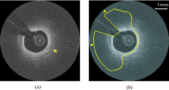
1.IntroductionCoronary calcified plaque (CP) is an important marker of atherosclerosis and can provide an estimate of total coronary plaque burden for a patient.1, 2, 3, 4, 5, 6 Although no clear relationship between calcification and plaque vulnerability has been established,4 an automatic method to segment and quantify CP in medical images would facilitate our understanding of its role in the clinical coronary heart disease (CHD) risk assessment.1 Moreover, heavily calcified lesions are often associated with a lower success rate of coronary stenting and require usage of additional devices, such as rotational atherectomy.7 Quantification of calcified lesions, such as their depth and thickness, can provide valuable information for guiding complex interventional strategies in vessels with superficial calcification. Both noninvasive and invasive methods can be used for CP detection and quantification. Noninvasive methods, such as multislice spiral computed tomography (MSCT)/multidetector CT (MDCT), and electron beam CT (EBCT), are the natural choices for general calcium-score evaluation,1, 3, 5, 6, 8 but their limited spatial resolution (∼1 mm) provides inadequate morphological lesion assessment. Invasive methods include intravascular ultrasound (IVUS)9, 10, 11 and optical coherence tomography (OCT).9 , 12, 13, 14 IVUS has a resolution of ∼200 μm and is able to detect CP, but cannot measure the distance between the superficial CP and the lumen, nor can it assess the thickness of CP due to the strong acoustic shadowing caused by calcium.11 Intracoronary OCT, with much higher resolution (10–20 μm), can provide detailed volumetric characterization of CP. It is also a powerful tool to study the association of CP with other noncalcified types of plaques with higher sensitivity and specificity.9, 14, 15 OCT is able to differentiate superficial CP from deep CP. The superficial CP is of primary clinical concern because it can result in underexpansion of the stent, which increases the risk of stent thrombosis. OCT image analysis has already become the most speed-limiting step in the CHD risk-evaluation process. This is because current OCT image analysis is still a frame-based process involving time-intensive manual image segmentation and quantification. Appropriate automatic image processing, if possible, would greatly increase the efficiency of image analysts, enabling them to focus on the more important decision-making tasks. One such example is the automatic lumen segmentation already utilized in commercial OCT systems (LightLab Imaging Inc., Massachusetts, Westford). Tearney performed automatic quantification of macrophages in OCT images16 and utilized this method in 3-D visualization of a coronary artery.17 But overall, few automatic image segmentation or quantification methods for intracoronary OCT applications were reported. In particular, no automatic methods are available for CP assessment by OCT. As intracoronary OCT is becoming a mature imaging modality for diagnosis of vulnerable plaques or evaluation of coronary stenting, rapid and accurate quantification of CP can greatly improve the efficiency of OCT-based CHD risk evaluation or stent intervention in clinical environments. The purpose of this study is to demonstrate a semiautomatic method for segmentation and quantification of CP in coronary artery OCT images. The method is “semiautomatic” because the starting and ending frames of the image stack containing CPs are manually preselected as the input to the algorithm. After segmentation, false-positive (FP) regions are manually removed by single mouse clicks. No manual input of initial contours or seed points are required nor are any training images needed. The design aims at minimizing operator interactions involved and serves as an important milestone toward a fully automatic approach. The method consists of a series of sequential procedures, including preprocessing, CP localization, CP segmentation, and postprocessing, and finally provides clinical relevant quantitative measures of CP, including depth, area, angle fill fraction (AFF), and thickness.11 2.Experimental Methods2.1.OCT ImagesImages used in this study were collected by LightLab prototype Fourier-Domain OCT (FDOCT) systems (CV-M4, LightLab Imaging Inc., Massachusetts). The system is equipped with a tunable laser light source with a center wavelength of 1310 nm and full-width-at-half-maximum bandwidth of 80 nm, providing ∼15-μm axial resolution in air. The lateral resolution is ∼30 μm. The scan characteristics of the M4 system are 100 fps, 45,000 lines/s, 456 lines/frame, 20-mm/s pullback, and 5-mm scan range in air (3.8 mm in saline). All the intracoronary OCT images were acquired from the database in the image reading center at the Core Lab (Harrington-McLaughlin Heart & Vascular Institute, University Hospitals Case Medical Center, Cleveland, Ohio). Stents were implanted in a large spectrum of clinical presentations varying from asymptomatic to acute myocardial infarction patients. OCT images from nine pullbacks (eight patients) were arbitrarily selected from our database. Out of these images, only nonstented segments containing CPs were selected (∼10% of the total images). Frames with substantial luminal blood, unclear lumen, or inadequate contrast for CP recognition by human observers were excluded. This gave a total of 106 images used for analysis and validation. The rectangular-view raw data, instead of the end-user polar-view images provided by the LightLab workstation, were log transformed and then used as the starting point for automatic image analysis. 2.2.Manual Classification of CPsCPs were manually detected and classified for further validation experiments. The signal-poor regions and sharply delineated borders,15 as shown in Fig. 1, are the two primary features of CP. One limitation of the current intravascular OCT system is that the imaging probe is delivered by a standard guide wire, which may block the CP being imaged. Depending on the guide wire's position, CPs are classified as GW0 if not blocked [Fig. 1, 8 and 12 o’clock], GW1 if they only appear on one side of the guide-wire shadow [Fig. 1, 3–5 o’clock], and GW2 if they appear on both sides of the shadow [Fig. 1]. We name the near-lumen CP border as the inner border (IB), and the far-lumen CP border as the outer border (OB) (Fig. 1). Because of the limited penetration depth of infrared light, the CP is categorized as C-OB if its OB is clear, and UnC-OB if the arc of its unclear part OB is ≥30 deg (the center of the arc is the centroid of lumen). CPs blocked by the guide wire or having unclear OB impose additional challenges for manual and automatic segmentation. Fig. 1Polar OCT images containing CPs. IB is near the lumen (arrows) while OB is far from the lumen (arrow heads). Stars refer to the guide wire. (a) CPs with clear OB. The CP at 3–5 o’clock is partially blocked by the guide wire (GW1). (b) The OB of a large CP is clear from 7 to12 o’clock, but is obscured from 12 to 2 o’clock. The CP is truncated by the guide wire shadow at 12–1 o’clock (GW2).  2.3.Validation ExperimentsTwo independent expert OCT image observers blinded to automatic segmentation results were involved in the manual contour tracing process, which was performed on commercial LightLab OCT workstations. OCT observer 1 finished all 106 images, while OCT observer 2 randomly analyzed 63 of the 106 images. The 63 images were used to evaluate interobserver and computer-observer variability. Automatic and manual segmentation results were compared using a Dice coefficient (DSC), defined as DSC = 2|A∩M|/(|A| + |M|), where A and M are the automatic and manual binary segmentation results, respectively. A more stringent metric, Hausdorff distance19 was also used to assess the performance. It is defined as the maximum of the set of minimum distances between the points on two boundaries. The Williams Index (WI)19 was utilized to evaluate the ratio of the average human-human agreement to the average computer-human agreement. Quantitative parameters derived from the automatic and manual segmentation results were compared, and the mean and standard deviation of the differences were reported. 3.Image Analysis AlgorithmFigure 2 summarizes the entire image analysis algorithm. After the preprocessing steps, including segmentation of the lumen, guide wire, and arterial wall, the CP was localized by edge detection and traced using a combined intensity and gradient-based level-set model. Postprocessing and quantification were then performed based on the segmentation results. Fig. 2Flowchart of the entire method. Following segmentation of the lumen, guide wire, and arterial wall, the CP was localized by edge detection and traced using an active contour model. Quantification was performed based on the segmentation results.  3.1.Preprocessing3.1.1.Lumen segmentationA binary image was generated from the input rectangular view image using Otsu's automatic thresholding method,18 and this produced three large structures: the arterial wall, the guide wire, and the sheath of the catheter. The guide wire and catheter sheath were removed by applying an area constraint (i.e., any isolated region with an area smaller than a threshold was removed). A morphological closing was used to fill in small holes inside the arterial wall, generating a bright superficial layer (BSL), the polar view of which was shown in Fig. 3. The border of the lumen was easily identified by searching the first BSL pixel in the light-propagation direction along each A scan in the rectangular view. The lumen edge may break into several segments due to presence of guide wire or side branches. The piecewise border of the lumen was connected by interpolation of the missing border, which became a smooth contour after polar transformation [Fig. 3]. 3.1.2.Guide wire segmentationThe guide wire is highly reflective and manifests itself in OCT images as a bright body protruding into the lumen with a long shadow behind it (Fig. 1). Our guide-wire segmentation technique exploits these two characteristics. It can be seen that the guide-wire shadow is a gap in the BSL. If more than one gap is present (e.g., a side branch), then the gap with the brightest pixels (guide-wire body) along the A lines within the gap is considered to be the guide-wire shadow. If the guide wire is misidentified in an individual frame, then the detected guide-wire position of individual frames can be reconciled by morphological opening along the longitudinal direction. After the guide wire is detected, all the A lines of the guide-wire shadow are excluded from further analysis. 3.1.3.Arterial wall segmentationAdventitia is commonly, but not always, seen in OCT images, depending on the thickness of intima and the presence of plaques. The presence of CP will hide the adventitia interface [Fig. 4] due to light attenuation. The aim of arterial wall segmentation is to exclude the adventitia tissue from the CP search region because adventitia may generate FP responses in CP localization. Apart from relatively low intensity and edge information, which may be shared by CP as well, the unique texture was used to exclude adventitia. We applied a texture-based level-set model following the work of Sandberg 19 and Cham and Vese.20 Texture information was extracted using Gabor filters19, 21 with five orientations (60, 75, 90, 105, and 120 deg; angles were with reference to the incident light). This resulted in five different texture images, which were incorporated into a vector-based energy function in the active contour model. The active contour framework was similar as that used in the CP segmentation step and will be discussed in detail in Section 3.3. The contour was initialized to the lumen contour as shown in Fig. 3; it evolved based on the texture information of the image and stopped at the boundary where the texture difference between the regions outside and inside the contour was maximized. Before arterial wall segmentation, the contour depth limit was set as ∼2 mm [Fig. 4]. 3.2.CP LocalizationThe localization was conducted in rectangular view images and based on edge detection, the purpose of which was also to provide a gradient image for the active contour model in the following segmentation step. Before edge detection, the original image was smoothed by a median filter to reduce speckle noise. A special matched filter22 was designed to detect the CP boundary [Fig. 5]. The edge detection was performed in a sequential approach. First, the strong IB in the rectangular view was detected by the filter rotating from –15 to 15 deg by a 5-deg interval (angles were with reference to the incident light), and the maximum response at each pixel was set as the final gradient value for that pixel, thereby generating a gradient image. A binary edge mask was obtained by hysteresis thresholding.23 A horizontal Prewitt operator was then used to fix any possibly missed extremely shallow IB with a depth smaller than the size of the matched filter. The gradient image for OB was obtained following the same procedure but by the filter oriented along different directions. The corresponding binary edge image was generated such that only the edges connected to or were behind the IB were included. The final gradient image and binary edge image were obtained by combining the individual responses from IB and OB together [Fig. 5]. Fig. 5(a) The matched filter used for edge detection. (b) Binary edge image. The edges of the guide wire detected in the guide wire segmentation step were also kept for making up the GW1/2 CP edge that was blocked by the guide wire. (c) The initial contour generated from the binary edge image by morphological dilation.  After edge detection, the Region of Interest (ROI) was updated by locating edge aggregations along the arterial wall. Once the binary edge area within a 40-deg segment translating the vessel wall exceeded a threshold of 0.02 mm2, the segment was marked as the initial ROI. The segment length was increased until there was no change in edge intensity and was stored as the final ROI for the CP. 3.3.CP Segmentation Based on an Active Contour ModelWe used a level-set approach based on the work of Li 24 and Chan and Vese.20 The initial contour was created from the polar transformed binary edge image by morphological dilation [Fig. 5]. We define ϕ as a signed distance function (SDF) with its zero-level curve represented by C = {(x, y)|ϕ = 0}. ϕ < 0 if ϕ is outside C and ϕ > 0 if ϕ is inside C. The initial contour C 0 is driven to the desired CP boundary by minimizing the following energy term: Eq. 1[TeX:] \documentclass[12pt]{minimal}\begin{document}\begin{eqnarray} E &=& \mu \int_\Omega {\frac{1}{2}} (\nabla \phi - 1)^2 dxdy\,{+}\,\lambda \int_\Omega {g'\delta (\phi)| {\nabla \phi}|} dxdy\nonumber\\ &&{+}\,\upsilon\!\int_\Omega {g'H(-\phi)}dxdy\,{+}\,\kappa\!\left(\int_\Omega\! {| {I_0 (x,y)\,{-}\,c_1}|^2 H(\phi)} dxdy\right. \!\nonumber\\ &&\left.{+}\,\int_\Omega \!{| {I_0 (x,y) -\! c_2} |^2 (1 \!- \!H(\phi))}dxdy \!\right),\!\! \end{eqnarray}\end{document}The evolving contour was stopped if it hit the boundary in the binary edge image and its speed was close to zero. Unlike traditional level-set methods, the starting contour C 0 was initialized not as one SDF but as nSDFs, where n was the number of separate regions in C 0. The stopping criterion for every SDF was evaluated separately. Each SDF used the same parameters, defined above, and evolved independently. Because of the flexible topology of the level set and the positive value of the area term, existing SDFs could have broken into multiple contours. In these cases, each separate contour was reinitialized into a daughter SDF and began its own evolution. Because tiny calcified lesions are assumed to be of little clinical relevance, any contour islands <0.03 mm2 were removed during the contour evolution process. A slightly different energy function [Eq. 2] was used for arterial wall segmentation in Section 3.1.3, Eq. 2[TeX:] \documentclass[12pt]{minimal}\begin{document}\begin{eqnarray} E &=& \mu _{\rm a} \int_\Omega {\frac{1}{2}} (\nabla \phi - 1)^2 dxdy + \lambda _{\rm a} \int_\Omega {\delta (\phi)\left| {\nabla \phi} \right|} dxdy\nonumber\\ && +\, \upsilon _{\rm a} \int_\Omega {\frac{1}{{1 + {\rm DM}}}H(- \phi)} dxdy\nonumber\\ && +\, \kappa _{\rm a} \left(\frac{1}{N}\sum\limits_{i = 1}^N \left\{\int_\Omega {\big| {T_{0}^i (x,y) - c_{1}^i} \big|^2 H(\phi)} dxdy\right.\right.\nonumber\\ &&+\,\left.\left. \int_\Omega \left| T_{_0}^i (x,y) - c_{_2}^i \right|^2 [1 - H(\phi)] dxdy \right\} \right). \end{eqnarray}\end{document}3.4.PostprocessingIf there were segmented regions on both sides of the guide-wire shadow, the gap between the two separate regions was padded by interpolation to restore the part of the CP blocked by the guide wire (case GW 2). Because it is very unlikely for a CP to appear in one single frame, any CP that did not appear in adjacent frames was removed. All the longitudinally connected regions were labeled as one CP, and other unconnected regions in individual frames were labeled in a clockwise order, starting from 12 o’clock. FP regions were manually removed before the validation and quantification. 3.5.QuantificationFour quantitative measures, the depth, area, thickness, and AFF were calculated automatically. The calculation of area was trivial. The depth, thickness, and AFF were all calculated with reference to the centroid (indicated by O) of the lumen for each individual CP. Figure 6 illustrates the methodology. The depth and thickness are defined as Eq. 3[TeX:] \documentclass[12pt]{minimal}\begin{document}\begin{equation} {\rm Depth} = \frac{1}{n}\sum\limits_i^n {D_{i\;\;}} \;\;{\rm Thickness} = \frac{1}{n}\sum\limits_i^n {T_i}, \end{equation}\end{document}Fig. 6Quantification metrics. The yellow dotted lines radiating from the centroid of the lumen serve as the direction along which the depth and thickness are measured. The red and green double arrows indicate the depth and thickness measurement, respectively. AFF is the largest angle between the rays across the CP boundaries. (Color online only.) 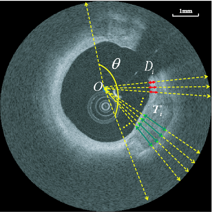 4.Results4.1.Determination of Algorithm ParametersAll the input images or intermediate images used during the image processing were normalized to the 0–1 range. All the thresholds used in the method were either represented in absolute unit, which was proportional to the size of the original image, or in relative unit, represented by r%, indicating that the brightest r% pixels of the original images were kept after thresholding. Suppose the size of the input raw image (rectangular view) was M×N, the size of the polar transformed image was P×P, we generally chose the area constraint used in the lumen segmentation to be 0.016MN. The intensity threshold for edge detection was 1%, and the threshold for capturing the edge aggregations was set as 0.002MN. The coefficients of the energy terms in the CP segmentation and the arterial segmentation steps were chosen as follows: w = 0.02P, μ = 0.02, λ = 20, υ = 1, and κ = 5 if there was no overlap between the evolving contour and the lumen; κ = 0 otherwise, w a = 0.08P, μa = 0.02, λa = 15, υa = −15, and κa = 100. 4.2.Lumen Segmentation and Guide Wire SegmentationAlthough lumen segmentation and guide-wire segmentation are not the primary focus of this study, they do serve as the basis for CP segmentation and quantification. Comparison between automatic lumen segmentation and semiautomatic lumen tracing on LightLab OCT workstations (automatic lumen tracing with manual postcorrection) revealed high accuracy (Table 1). The performance of the guide-wire segmentation was evaluated by observation. The segmentation result was considered correct if the detected guide-wire shadow agreed with the real position. An accuracy of 100% was achieved. Table 1Lumen and guide wire segmentation results.
4.3.CP Segmentation, Validation, and QuantificationOut of the 106 images, a total of 138 CPs were identified and traced by both human observers. The algorithm segmented all the CPs, but also gave 88 FP regions. All the longitudinally connected FPs were removed at once by a single mouse click on the FP regions. Figure 7 shows three examples of automatic segmentation results. Figure 7 contains three CPs with clear OB. Although the CP at 3–4 o’clock is partly blocked by the guide wire, the effect on the automanual agreement is negligible. We show in Fig. 7 that our method can guess and approximate the part of the CP blocked by the guide wire. A FP region is also shown at 1–2 o’clock. We next demonstrate the performance of the method on a large CP with irregular shape and unclear OB [Fig. 7]. A large disagreement between humans and computer appears on the OB. Fig. 7(a–c) Original images and (d–f) corresponding manual and automatic segmentation results. Red: observer 1; blue: observer 2; yellow: automatic method. The CPs in (a) and (b) have clear OB, and the CP in (c) has unclear OB. The CPs in (b) and (c) are blocked by the guide wire. A false positive region is also shown in (e). (Color online only.) 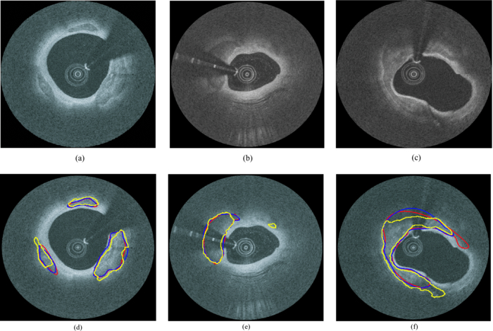 We evaluated the performance of the method on different categories of CP as shown in Fig. 8. Out of the 138 CPs, 48 of them were blocked by the guide wire (GW2) and 77 of them had unclear OB. The DSC for C-OB is significantly higher than UnC-OB (unpaired Student's t-test: P < 0.01). The method also performed better on GW0/GW1 than on GW2 (P < 0.01). The overall DSC for all the CPs is 0.78 ± 0.09. In comparison, the DSC between two human observers is 0.89 ± 0.07. Fig. 8Dice coefficient for CPs with or without a clear outer border (C-OB or UnC-OB), blocked (GW1, GW2), or not blocked (GW 0) by the guide wire, and total. *P < 0.01 (unpaired Student t-test).  Figure 9 shows the WI calculated based on DSC and Hausdorff distance (HD), respectively. The higher WI for C-OB compared with UnC-OB, and that for GW0/GW1 compared with GW2 indicates that there is more disagreement between computer and humans than human and human for UnC-OB and GW2. However, an overall WI of 0.85 for DSC and 0.7 for HD suggest reasonable agreement between the automatic and manual segmentation. Fig. 9WI calculated from (a) Dice coefficient and (b) Hausdorff distance. If WI is close to 1, then the agreement between the automatic method and humans is close to that between humans. 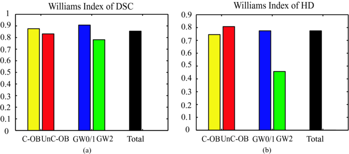 Because there is a large interobserver variability for UnC-OB or GW2 CP segmentation, we only performed quantification in CPs with a clear outer border and no guide-wire overlap (42 CPs). Individual measurements of each CP are shown in Fig. 10. The area, AFF, and thickness of the CPs have a large distribution, while the depth is constrained within a shallow layer under the lumen. Table 2 gives the unsigned and signed differences between the automatic and manual method in both absolute and relative units. Overall, accuracies >80% are achieved for all the quantitative measurements except for the depth measurement, which results in a 23.9% unsigned error. Also, there is insignificant bias except the depth measurement. Figure 10 indicates that the automatic method tends to overestimate the depth of very superficial CPs. Fig. 10Quantification results for each CP with clear outer border and no guide wire overlap: (a) Area, (b) AFF, (c) depth, and (d) thickness.  Table 2Mean ± standard deviation of quantitative measurement differences between the automatic and manual method for CPs with clear outer border and no guide wire overlap.
4.4.3-D VisualizationFigure 10 shows a 3-D rendered coronary artery segment from one of the data sets used in this study. A comparison between the manual and automatically rendered CP was shown in Figs. 10 and 10. Although there are segmentation errors in single frames, automatically rendered CP does not differ significantly from the manual result. 5.Discussion5.1.Limitations of CP Segmentation and Potential ImprovementIn clinical applications, OCT images can be noisy, bad quality, or simply do not exhibit the typical tissue characteristics discussed above. We evaluate some possible circumstances when each part of the algorithm might fail and provide corresponding strategies if possible. 5.1.1.Lumen segmentationThe catheter may be erroneously identified as vessel wall when they are in contact with each other. One approach to correct the catheter artifact is to apply prior information of the catheter size. A more complicated case is when there is substantial luminal blood in contact with the arterial wall. If so, manual interaction is required. 5.1.2.Arterial wall segmentationIf the adventitia exists but does not exhibit the typical texture similar to that shown in Fig. 4, the arterial wall segmentation algorithm may fail and FP may be generated. Research is being conducted to develop a more robust method for arterial wall segmentation. For example, more texture features of the adventitia can be included and built into a classification scheme and the smoothness of the contour in 3-D space also adds more information. 5.1.3.CP edge detectionWhen most of the CP IB is in contact with the lumen border, the edge-detection algorithm may fail because the IB could not be differentiated from the lumen border. Under such circumstances, users may provide some auxiliary points on the IB to help the algorithm identify the CP. 5.1.4.Level-set segmentationThe algorithm tends to fail around the connecting region between the IB and OB. The CP boundary here is usually blurred due to its relatively parallel direction to the incident light and is even completely missing in some cases [e.g., Fig. 7]. Often, this region extended into the surrounding tissue without intensity changes and neither the gradient term nor the intensity term could easily stop the algorithm at the desired boundary. As shown in Figs. 8 and 9, the algorithm also performs less satisfactorily for GW2 or UnC-OB, which are also difficult for humans, as indicated by the relatively low DSC between the two observers (0.88±0.07 for GW2 and 0.86±0.06 for UnC-OB). Collectively, these results indicate that unlike lumen segmentation, the CP segmentation is intrinsically much more complex. 5.1.5.FP generationOne limitation of our automated segmentation is the occurrence of FP, which may result from oversensitive parameters set in the edge-detection procedure and also because the tissue structures have similar appearances as CP. Figure 7 gives such an example. The FP has a similar dark region as CP but with a more diffuse border. Its specific tissue type remains unknown due to the lack of histology. Besides such unknown dark structures, side branches and small pieces of adventitia tissue without the typical texture shown in Fig. 4 may also cause FPs. In our method, removal of FPs was performed manually with a single mouse click. This does not complicate the process significantly because all longitudinally connected regions can be removed at once. Additional analysis may enable achievement of full automation. One possibility is post-tissue classification using image features extracted from the isolated segmented regions to remove FPs. Or, a separate automatic CP detection technique may be considered. 5.2.Quantification and 3-D Volumetric AnalysisWe demonstrated that coronary CPs with clear OB and no guide-wire overlap can be quantified automatically with adequate accuracy. The absolute unsigned error of the automatic depth measurement is only 0.04±0.04 mm, approximately twice as much as the OCT resolution. However, this represents a relative error of 23.9±23.9% because the average depth is only 0.17±0.09 mm. When the IB protrudes into the luminal surface, the estimated border is always below the luminal boundary, thus resulting in a large signed error of the automatic depth measurement. As for other measures, the AFF is analogous to the calcium arc used in IVUS.11 The area serves as the basis for 3-D volumetric analysis (Fig. 11). In our method, the lumen, guide wire, and CP are all segmented automatically, enabling automated 3-D rendering of an entire calcified coronary artery segment within seconds, which is practical for the clinical environment. Fig. 113-D rendering of a volumetric OCT image set: (a) 3-D rendering from manual segmented CP and (b) 3-D rendering from automatic segmented CP. Lumen and guide wire are automatically segmented in both (a) and (b). (c, d) Fly-through view of automatic segmentation results at different zoom levels. White: CP; blue: guide wire; and orange: coronary arterial wall. The intima layer blocked by the guide wire is not rendered, while the underlying CP is rendered.  5.3.Clinical ImplicationsIt is generally accepted that coronary artery calcification increases with the extent and severity of atherosclerosis, and its progression may correspond with cardiovascular event rates.1, 2, 3, 4, 5 , 11 Currently, the coronary calcium score calculated by multiplying the CP area by an X-ray attenuation coefficient8 is routinely evaluated by cardiac CT to predict the total plaque burden of a patient. With superior resolution and the ability to penetrate calcium, OCT provides the potential for more precise volumetric calcium assessment. Furthermore, in addition to the numerical calcium score, the morphological information as provided by OCT may reveal more about the role of calcification associated with atherosclerosis. Automatic segmentation and quantification will be important for volumetric calcium assessment by OCT. Superficial CP plays a determinant role in successful stent deployment. Compared to IVUS and CT, OCT has the unique capability to quantify the depth and thickness of superficial CP. Over half the CPs involved in this study had a depth lower than the resolution of IVUS (<0.2 mm). The thickness of most CPs was <0.7 mm [Fig. 10], which could not be resolved by CT. As an example, the spatial resolution of the EBCT and MDCT used in the large multi ethnic study of atherosclerosis (MESA) was 0.68×0.68×3.00 mm and 0.68×0.68×2.50 mm,26 respectively. Superficial CP may cause underexpansion of the stent, but what degree of superficial CP requires additional treatment remains unknown. The thickness of CP directly determines whether rotational atherectomy should be used to expand the vessel before coronary stenting and therefore affects the success rate associated with the procedure. Automatic CP quantification by OCT brings new information for interventional strategies, especially for a decision on the necessity of rotational atherectomy. Another application of our method is for plaque characterization. A recent study27 has shown that different types of plaques (fibrous, lipid, and calcified) can be classified based on combined backscattering and attenuation coefficients. An important prerequisite for accurate plaque characterization is that individual plaque types should be isolated for fitting the first-order scattering model.27, 28 In addition, some plaques are in nature mixed together (e.g., fibrocalcified plaque). The automatic segmentation of CP may facilitate the automation of the plaque characterization process. 5.4.ConclusionsWe demonstrated for the first time that the coronary CP in OCT images can be segmented and quantified by the proposed semiautomatic method. This will contribute to the general volumetric calcium assessment and superficial calcium evaluation for necessity of rotational atherectomy before percutaneous coronary intervention. AcknowledgmentsThe authors thank Wei Kang, Michael Jenkins, Zhilin Hu, Anagha Deshmane, and Stan Pokras for valuable discussions. ReferencesP. Greenland,
R. O. Bonow,
B. H. Brundage,
M. J. Budoff,
M. J. Eisenberg,
S. M. Grundy,
M. S. Lauer,
W. S. Post,
P. Raggi,
R. F. Redberg,
G. P. Rodgers,
L. J. Shaw,
A. J. Taylor,
W. S. Weintraub,
R. A. Harrington,
J. Abrams,
J. L. Anderson,
E. R. Bates,
C. L. Grines,
M. A. Hlatky,
R. C. Lichtenberg,
J. R. Lindner,
G. M. Pohost,
R. S. Schofield,
S. J. Shubrooks Jr., J. H. Stein,
C. M. Tracy,
R. A. Vogel, and
D. J. Wesley,
“ACCF/AHA 2007 Clinical Expert Consensus Document on Coronary Artery Calcium Scoring by Computed Tomography in Global Cardiovascular Risk Assessment and in Evaluation of Patients with Chest Pain: A Report of the American College of Cardiology Foundation Clinical Expert Consensus Task Force (ACCF/AHA Writing Committee to Update the 2000 Expert Consensus Document on Electron Beam Computed Tomography), Developed in Collaboration with the Society of Atherosclerosis Imaging and Prevention and the Society of Cardiovascular Computed Tomography,”
J. Am. Col. Cardiol., 49
(3), 378
–402
(2007). https://doi.org/10.1016/j.jacc.2006.10.001 Google Scholar
L. Wexler,
B. Brundage,
J. Crouse,
R. Detrano,
V. Fuster,
J. Maddahi,
J. Rumberger,
W. Stanford,
R. White, and
K. Taubert,
“Coronary artery calcification: pathophysiology, epidemiology, imaging methods, and clinical implications: a statement for health professionals from the American Heart Association,”
Circulation, 94
(5), 1175
–1192
(1996). Google Scholar
M. J. Pletcher,
J. A. Tice,
M. Pignone, and
W. S. Browner,
“Using the coronary artery calcium score to predict coronary heart disease events: a systematic review and meta-analysis,”
Arch. Intern. Med., 164
(12), 1285
–1292
(2004). https://doi.org/10.1001/archinte.164.12.1285 Google Scholar
A. P. Burke,
D. K. Weber,
F. D. Kolodgie,
A. Farb,
A. J. Taylor, and
R. Virmani,
“Pathophysiology of calcium deposition in coronary arteries,”
Herz, 26
(4), 239
–244
(2001). https://doi.org/10.1007/PL00002026 Google Scholar
R. Detrano,
A. D. Guerci,
J. J. Carr,
D. E. Bild,
G. Burke,
A. R. Folsom,
K. Liu,
S. Shea,
M. Szklo,
D. A. Bluemke,
D. H. O'Leary,
R. Tracy,
K. Watson,
N. D. Wong, and
R. A. Kronmal,
“Coronary calcium as a predictor of coronary events in four racial or ethnic groups,”
N. Engl. J. Med., 358
(13), 1336
–1345
(2008). https://doi.org/10.1056/NEJMoa072100 Google Scholar
R. A. Kronmal,
R. L. McClelland,
R. Detrano,
S. Shea,
J. A. Lima,
M. Cushman,
D. E. Bild, and
G. L. Burke,
“Risk factors for the progression of coronary artery calcification in asymptomatic subjects: results from the multi-ethnic study of atherosclerosis (MESA),”
Circulation, 115
(21), 2722
–2730
(2007). https://doi.org/10.1161/CIRCULATIONAHA.106.674143 Google Scholar
I. Moussa,
C. Di, J. Moses,
B. Reimers,
L. Di, G. Martini,
J. Tobis, and
A. Colombo,
“Coronary stenting after rotational atherectomy in calcified and complex lesions: Angiographic and clinical follow-up results,”
Circulation, 96
(1), 128
–136
(1997). Google Scholar
A. S. Agatston,
W. R. Janowitz,
F. J. Hildner,
N. R. Zusmer,
M. Viamonte Jr., R. Detrano,
“Quantification of coronary artery calcium using ultrafast computed tomography,”
J. Am. Col. Cardiol., 15
(4), 827
–832
(1990). https://doi.org/10.1016/0735-1097(90)90282-T Google Scholar
B. D. MacNeill,
H. C. Lowe,
M. Takano,
V. Fuster, and
I. K. Jang,
“Intravascular modalities for detection of vulnerable plaque: current status,”
Arterioscler. Thromb. Vasc. Biol., 23
(8), 1333
–1342
(2003). https://doi.org/10.1161/01.ATV.0000080948.08888.BF Google Scholar
M. D. Baumgart,
M. A. Schmermund,
M. G. Goerge,
M. M. Haude,
M. J. Ge,
M. M. Adamzik,
M. C. Sehnert,
M. K. Altmaier,
M. D. Groenemeyer, and
M. R. Seibel,
“Comparison of electron beam computed tomography with intracoronary ultrasound and coronary angiography for detection of coronary atherosclerosis,”
J. Am. Col. Cardiol., 30
(1), 57
–64
(1997). Google Scholar
G. S. Mintz,
J. J. Popma,
A. D. Pichard,
K. M. Kent,
L. F. Satler,
Y. C. Chuang,
C. J. Ditrano, and
M. B. Leon,
“Patterns of calcification in coronary artery disease: a statistical analysis of intravascular ultrasound and coronary angiography in 1155 lesions,”
Circulation, 91
(7), 1959
–1965
(1995). Google Scholar
D. Huang,
E. A. Swanson,
C. P. Lin,
J. S. Schuman,
W. G. Stinson, and
W. Chang,
“Optical coherence tomography,”
Science, 254 1178
–1181
(1991). https://doi.org/10.1126/science.1957169 Google Scholar
I.-K. Jang,
B. E. Bouma,
D.-H. Kang,
S.-J. Park,
S.-W. Park,
K.-B. Seung,
K.-B. Choi,
M. Shishkov,
K. Schlendorf,
E. Pomerantsev,
S. L. Houser,
H. T. Aretz, and
G. J. Tearney,
“Visualization of coronary atherosclerotic plaques in patients using optical coherence tomography: comparison with intravascular ultrasound,”
J. Am. Col. Cardiol., 39
(4), 604
–609
(2002). https://doi.org/10.1016/S0735-1097(01)01799-5 Google Scholar
I. K. Jang,
G. J. Tearney,
B. MacNeill,
M. Takano,
F. Moselewski,
N. Iftima,
M. Shishkov,
S. Houser,
H. T. Aretz, and
E. F. Halpern,
“In vivo characterization of coronary atherosclerotic plaque by use of optical coherence tomography,”
Circulation, 111
(12), 1551
–1551
(2005). https://doi.org/10.1161/01.CIR.0000159354.43778.69 Google Scholar
H. Yabushita,
B. E. Bouma,
S. L. Houser,
H. T. Aretz,
I. K. Jang,
K. H. Schlendorf,
C. R. Kauffman,
M. Shishkov,
D. H. Kang, and
E. F. Halpern,
“Characterization of human atherosclerosis by optical coherence tomography,”
Circulation, 106
(13), 1640
–1645
(2002). https://doi.org/10.1161/01.CIR.0000029927.92825.F6 Google Scholar
G. J. Tearney,
H. Yabushita,
S. L. Houser,
H. T. Aretz,
I.-K. Jang,
K. H. Schlendorf,
C. R. Kauffman,
M. Shishkov,
E. F. Halpern, and
B. E. Bouma,
“Quantification of macrophage content in atherosclerotic plaques by optical coherence tomography,”
Circulation, 107
(1), 113
–119
(2003). https://doi.org/10.1161/01.CIR.0000044384.41037.43 Google Scholar
G. J. Tearney,
S. Waxman,
M. Shishkov,
B. J. Vakoc,
M. J. Suter,
M. I. Freilich,
A. E. Desjardins,
W.-Y. Oh,
L. A. Bartlett,
M. Rosenberg, and
B. E. Bouma,
“Three-dimensional coronary artery microscopy by intracoronary optical frequency domain imaging,”
J. Am. Col. Cardiol, 1
(6), 752
–761
(2008). Google Scholar
N. Otsu,
“A threshold selection method from gray-level histograms,”
IEEE Trans. Syst. Man. Cybernet., 9
(1), 62
–66
(1979). https://doi.org/10.1109/TSMC.1979.4310076 Google Scholar
B. Sandberg,
T. F. Chan, and
L. Vese,
“A level-set and Gabor-based active contour algorithm for segmenting textured images,”
(2002). Google Scholar
T. F. Chan, and
L. A. Vese,
“Active contours without edges,”
IEEE Trans. Image Proc., 10
(2), 266
–277
(2001). https://doi.org/10.1109/83.902291 Google Scholar
D. Gabor,
“Theory of communication,”
J. Inst. Elec. Eng., 93 429
–457
(1946). Google Scholar
D. H. Friedman, Detection of Signals by Template Matching, Johns Hopkins University Press, Baltimore, MD
(1969). Google Scholar
J. Canny,
“A computational approach to edge detection,”
IEEE Trans. Pattern Anal. Mach. Intell., 8
(6), 679
–698
(1986). https://doi.org/10.1109/TPAMI.1986.4767851 Google Scholar
C. Li,
C. Xu,
C. Gui, and
M. Fox,
“Level set evolution without re-initialization: A new variational formulation,”
430
–436
(2005) Google Scholar
T. F. Chan,
B. Y. Sandberg, and
L. A. Vese,
“Active contours without edges for vector-valued images,”
J. Vis. Commun. Image Represent., 11
(2), 130
–141
(2000). https://doi.org/10.1006/jvci.1999.0442 Google Scholar
J. J. Carr,
J. C. Nelson,
N. D. Wong,
M. McNitt-Gray,
Y. Arad,
D. R. Jacobs Jr., S. Sidney,
D. E. Bild,
O. D. Williams, and
R. C. Detrano,
“Calcified coronary artery plaque measurement with cardiac CT in population-based studies: standardized protocol of multi-ethnic study of atherosclerosis (MESA) and coronary artery risk development in young adults (CARDIA) study,”
Radiology, 234
(1), 35
–43
(2005). https://doi.org/10.1148/radiol.2341040439 Google Scholar
C. Xu,
J. M. Schmitt,
S. G. Carlier, and
R. Virmani,
“Characterization of atherosclerosis plaques by measuring both backscattering and attenuation coefficients in optical coherence tomography,”
J. Biomed. Opt., 13
(3), 034003
–034008
(2008). https://doi.org/10.1117/1.2927464 Google Scholar
J. M. Schmitt,
A. Knüttel, and
R. F. Bonner,
“Measurement of optical properties of biological tissues by low-coherence reflectometry,”
Appl. Opt., 32
(30), 6032
–6042
(1993). https://doi.org/10.1364/AO.32.006032 Google Scholar
|
|||||||||||||||||||||||||||||||||||||||