|
|
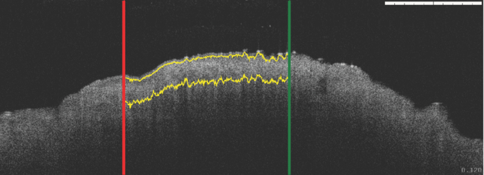
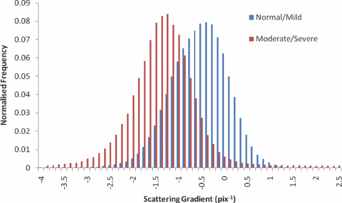
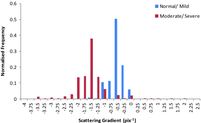
1.IntroductionObtaining an accurate histopathological diagnosis for oral epithelial dysplasia (OED) is dependent on the selection of the most representative site to biopsy. Today, identification of these sites can be a challenging procedure owing to the considerable variations in the clinical appearances of lesional and nonlesional locations. To facilitate improved localization of biopsy sites, techniques have been introduced for visualizing structural and metabolic alterations not revealed during clinical examinations. Such techniques include topical application of optical contrast agents such as toluidine blue,1 direct visualization of tissue fluorescence,2 and direct oral microscopy.3 Although these approaches have reported improved detection of abnormal areas, they remain limited by their dependence on static and qualitative assessment of disease sites.4 To obviate some of these issues, optical coherence tomography (OCT) should be considered. OCT is an emerging noninvasive imaging modality capable of producing quantitative assessment of tissue properties.5 For in vivo clinical evaluation of tissue it provides promising attributes, such as acquisition speed, imaging depth, micrometer-scale resolution, and 3-D sampling ability.6, 7 However, it lacks the resolution to provide the subcellular detail necessary for the interpretation of conventional histopathology images. Despite this, OCT was used in vivo to study oral dysplasia and malignancy in a hamster model,8, 9 revealing a correlation between gross morphological features in both OCT images and histological sections. Wilder-Smith more recently extended this work to a human study involving 50 patients,10 reporting differentiation of normal, dysplastic, and squamous cell carcinoma of the oral mucosa. These studies identified the potential of OCT to provide early detection and regular monitoring of suspect lesions in the oral cavity. However, the lack of subcellular detail in OCT and the dependence on subjective visual evaluation limits the absolute diagnostic efficacy. For example, a double-blinded clinical study of esophageal tissue by Isenberg 11 used endoscopic OCT to identify dysplasia in patients with Barrett's esophagus. It was concluded that OCT may be useful for directing biopsy toward dysplastic regions, but conceded that without further identification of OCT characteristics for dysplasia, the clinical applicability of OCT is presently limited. Hence, it is increasingly clear that there is limited clinical value in traditional B-scan mode visualization of OCT images for the identification of premalignancy. Accordingly, a multimodal imaging strategy was proposed, by combining OCT with Doppler and nonlinear microscopy techniques.12 While such a strategy approaches the sensitivity and specificity of conventional methods, the experimental configuration is large, complex, and not presently amenable to routine clinical use. A more valuable approach is to parameterize the acquired OCT data and thereby present an en face microscopy view of the tissue surface, onto which a quantitative marker of tissue health is mapped. The potential to parameterize OCT data was previously demonstrated by Levitz, 13 who measured the difference in scattering coefficient of both phantoms and tissue. Other studies have demonstrated the differentiation of plaque and arterial wall components using a similar approach.14 Of direct significance to this work is that of Tsai, 15 who proposed an empirical relationship between oral dysplasia and the rate of OCT signal decay as a function of depth. A similar analysis was also used to analyze oral submucous fibrosis with promising results,16 although it necessarily presents a wide variation in scattering gradients. This is often addressed by averaging A-scans over the transverse direction and obtaining a mean attenuation coefficient. However, subjective selection of a region over which the attenuation is estimated leads to further ambiguity in the analysis. A recent study by McLaughlin 17 implicitly addressed the former of these issues by spatially mapping the attenuation coefficient over a 3-D section of malignant human lymph node. Their results suggest that the wide variation in scattering coefficient derives from the heterogeneity of tissue. In this work, we develope a similar technique of spatially mapping the attenuation coefficient to image premalignant lesions of the oral mucosa. The method, termed scattering attenuation microscopy (SAM), defines an automated scheme for quantitative imaging of tissue attenuation from data obtained by OCT. 2.Theory2.1.OCTOCT is an optical imaging technique that employs low-coherence interferometry (LCI) to noninvasively form cross-sectional images (B-scans) of highly scattering samples. It has been widely reported in the literature for imaging biological specimens.18 B-scan images are comprised of a lateral series of sequential LCI axial scans (A-scans), each of which provides a measure of the incident light intensity scattered from morphological features within the sample back into the detection optics. A typical OCT instrument is composed of a broadband light source, a Michelson interferometer, and scanning optics by which images of the sample are obtained. For 3-D acquisition, frequency domain detection offers the required frame rates, using either spectrometer or swept laser source systems. A number of detailed reviews of OCT were previously published.19, 20 2.2.OEDThe normal oral mucosa is made up of two structurally distinct layers: an overlying epithelium and its underlying connective tissue, the lamina propria. In between these layers is the basement membrane, characterized by cells with increased nuclear size, and characterized in histology by high staining intensity (hyperchromatism). By contrast, mild, moderate, and severe dysplasias display basal-cell-like features in the bottom, middle, and upper third of the epithelium respectively. This re-distribution of cell nuclei is of particular relevance to OCT, which relies on the scattering of light to form cross-sectional B-scan images. The cell nuclei are a significant contributor to the light-scattering process. Therefore, any change in their spatial distribution or size will consequently affect the detected optical scattering profile in OCT. In human epithelial tissue, scattering dominates over optical absorption at a typical OCT imaging wavelength21 of 1300 nm. It follows that variations in the size and location of nuclear material in the epithelium will be exhibited as changes in the rate of axial intensity decay in OCT images. 2.3.Scattering Attenuation MicroscopyThe OCT A-scan signal I(z) from a homogeneous scattering medium, was previously described22 as a function of depth z, as shown by Eq. 1. This is valid in the limit of single scattering. Eq. 1[TeX:] \documentclass[12pt]{minimal}\begin{document}\begin{equation} I(z) = I_0 K\mu _b A(z){\kern 1pt} {\kern 1pt} \exp {\kern 1pt} {\kern 1pt}(- 2\mu _T z). \end{equation}\end{document}Eq. 2[TeX:] \documentclass[12pt]{minimal}\begin{document}\begin{equation} \mu _T = \mu _a + \mu _s. \end{equation}\end{document}OCT images are typically formed on a logarithmic intensity scale I log(z) = 20 log [I(z)], expressed in decibels (dB). For visualization, the logarithmic intensity is mapped to an 8-bit gray scale, Eq. 3[TeX:] \documentclass[12pt]{minimal}\begin{document}\begin{equation} I_{8{\rm bit}} (z) = 255\frac{{I_{\log } (z) - I_{\min } }}{{I_{\max } - I_{\min } }}, \end{equation}\end{document}Eq. 4[TeX:] \documentclass[12pt]{minimal}\begin{document}\begin{equation} I_{\log } (z) = \left\{ {\begin{array}{l@{\quad}l} {I_{\log } (z)} & {I_{\min } \le I_{\log } (z) \le I_{\max } } \\ {I_{\min}}, & {I_{\min } > I_{\log } (z)} \\ {I_{\max}}, & {I_{\log } (z) > I_{\max } } \\ \end{array}} \\ \right.. \end{equation}\end{document}Eq. 5[TeX:] \documentclass[12pt]{minimal}\begin{document}\begin{equation} I_{\rm 8bit} (z) = \ln \left[ {I_0 K\mu _b A(z)} \right] - \mu _T z - 255\frac{{I_{\min } }}{{I_{\max } - I_{\min } }}, \end{equation}\end{document}Eq. 6[TeX:] \documentclass[12pt]{minimal}\begin{document}\begin{equation} \epsilon = \frac{{255}}{{I_{\max } - I_{\min } }}\frac{{20}}{{\ln {} (10)}}. \end{equation}\end{document}Eq. 7[TeX:] \documentclass[12pt]{minimal}\begin{document}\begin{equation} \frac{\rm d}{{\rm d}z}I_{\rm 8bit} (z) = - \epsilon \mu _T. \end{equation}\end{document}2.4.Epithelial SegmentationAt tissue depths greater than [TeX:] $\mu _s^{ - 1},$ multiple scattering begins to dominate, and Eq. 1 is no longer a valid model. For human oral epithelium, [TeX:] $\mu _s^{ - 1}$ is typically23 of the order 0.5 mm, which is greater than its predicted thickness. The analysis should be focused within the epithelial tissues where the changes of interest are located. While automated segmentation of healthy epithelium is feasible with OCT images,24 the high attenuation associated with increasing severity of dysplasia prevents demarcation of the basement layer. Therefore, an alternative objective selection method was used, based on the percentage of backscattered light in the logarithmic domain. The integrated backscattered intensity from the surface to a depth [TeX:] $z_b$ is given by Eq. 8[TeX:] \documentclass[12pt]{minimal}\begin{document}\begin{equation} I_b (z_b)= \int\nolimits_0^{z_b } {I_{\log } (z)\;{\rm d}z}. \end{equation}\end{document}Eq. 9[TeX:] \documentclass[12pt]{minimal}\begin{document}\begin{equation} I_T = I_b (\infty). \end{equation}\end{document}3.Materials and MethodsApproval for this study was obtained from the ethics committee of Barts & the London Hospital, United Kingdom. Biopsy samples were obtained from 19 patients as part of the routine diagnostic procedure for suspected oral lesions. Biopsies were measured using OCT within 12 h of excision, after which they were sent to histopathology to be fixed, sectioned, stained and examined using standard histological procedures. OCT measurements were made using a commercial OCT microscope (EX1301, Michelson Diagnostics Ltd., United Kingdom) operating at a center wavelength of 1310 nm over a full width at half maximum (FWHM) spectral bandwidth of 75 nm. The axial and lateral FWHM resolution of this instrument were previously measured25 and found to be 10.9 ± 0.2 and 8.9 ± 0.2 μm, respectively. This instrument is composed of four interferometer channels, each focused with sequential axial offsets of 250 μm. Consequently, the depth-varying amplitude function A(z) in Eq. 1 is periodic between imaging depths of 0.0 to 0.7 mm, as shown in Fig. 3. To mitigate against the influence of this on the quantitative results, only the deepest focal channel was used. This was achieved by focusing the lower channel on the tissue surface. Therefore, the instrument was found to have a sensitivity drop of 25 dB over the selected portion of the OCT image depth that extended from 0.7 to 1.5 mm, as marked in Fig. 3 to the right of the dotted line. The peak channel sensitivity was measured to be 94±1 dB with an optical channel power of approximately 3 mW incident on the tissue surface. Fig. 3Sensitivity calibration curve for Michelson Diagnostics EX1301 OCT instrument used in this study. The dotted line coincides with the focus of the deepest channel.  Three-dimensional volumetric OCT data sets were obtained from sequences of B-scan images. Sequential images were acquired with a spacing of 5 μm using a computer-controlled linear translation stage (Z625B, Thorlabs Inc., United States). For each sample, the biopsy was orientated such that that the epithelial surface was presented to the OCT probe beam. Each A-scan in the 3-D volume was subjected to the segmentation and gradient assessment to determine a gradient value μ(x, y) at each orthogonal transverse position [x,y] over the volume surface. Hence, an en face view of the tissue attenuation parameter was obtained. For each sample, this was augmented by a histogram representing the statistical distribution of μ over the biopsy area. The units of μ are inverse pixels (pix−1), where the axial pixel spacing is 5.89 μm. 4.ResultsSamples were collated into two groups representing pathological assessments of normal/mild (15 biopsy specimens) and moderate/severe (4 biopsy specimens) dysplastic lesions. Analysis of each specimen comprised measurements of more than 100,000 A-Scans. 4.1.Normal/Mild DysplasiaFigure 4 shows results obtained from a fibroepithelial polyp used as a normal control in this study. The OCT image in Fig. 4 shows two distinct layers of signal intensity, representing epithelium (E) and superficial lamina propria (SLP). These closely match the anatomical layers in the corresponding histology [Fig. 4]. Fig. 4Normal control fibroepithelial polyp: (a) single OCT B-scan image, (b) corresponding histological section, (c) each point μ(x, y) contributes to the statistical distribution, and (d) multiple sequential OCT images contribute to an en face view of the sample, where the color map represents the spatial distribution of the scattering gradient μ(x, y).  4.2.Moderate/Severe DysplasiaFigure 5 shows results obtained from a moderately dysplastic oral mucosal biopsy sample. By contrast to Fig. 4, in Fig. 5 it is not possible to demarcate the tissue layers identified in Fig. 5. Therefore, Figs. 5 and 5 display poor morphologic correlation of the tissue layers in this sample. Fig. 5Typical example of moderate dysplasia. (a), (b), (c), and (d) are described for the normal control in Fig. 2.  4.3.Quantitative AnalysisThe histograms displayed in Figs. 4 and 5 represent statistical distributions of the gradient values for representative biopsy samples from each group. Contributing gradients were obtained from each transverse location [x,y] in the 3-D OCT data. Figure 4 shows a typical scattering gradient histogram for a single specimen from the normal/mild sample group. Likewise, Fig. 5 shows a scattering gradient histogram for a specimen from the moderate/severe group that exhibits a modal shift of −1.000 pix−1 (increased scattering) compared to the normal/mild group. Figure 6 shows scattering gradient histograms composed of every A-scan utilized for SAM imaging from all 19 biopsies. These represent 2 approximately normal distributions with distinct peaks at −0.4 and −1.3 pix−1 for normal/mild and moderate/severe, respectively, representing a similar scattering gradient change of 0.9 pix−1 to the individual samples. In Fig. 7, each B-scan is represented by its mode-scattering gradient, and these values are pooled into a histogram of all B-scans from all specimens. The mode rather than mean scattering gradient was chosen because the distribution of values within individual B-scans were found to be asymmetric. This may be due to the presence of multiple dysplastic severities present within a tissue section. 4.4.SAM Colour MapsIn Figs. 4 and 5, the gradient values are projected onto the biopsy sample surface, giving an en face view of the gradient heterogeneity. Gradient values between −3.0 and 0.0 pix−1 were encoded by a color map, representing 90% of acquired A-scan values. An upper value of 0.0 pix−1 was chosen because positive scattering gradients represented 23% of all normal/mild A-scans, compared with only 4% of all moderate/severe A-scans. Less than 0.1% of normal/mild A-scans exhibited scattering gradients below the lower bound of −3.0 pix−1. Therefore, the color map was configured such that a high degree of color homogeneity was observed in the normal/mild group [Fig. 4] and the moderate/severe group [Fig. 4] displayed significant color variation. 5.DiscussionThe poor morphologic correlation of tissue layers in Figs. 5 and 5 is due to increased optical scattering from dysplastic cells.26 The consequent morphological differences between Figs. 4 and 5 demonstrate the feasibility of qualitative differentiation using OCT. These OCT B-scans and corresponding histology [Figs. 4 and 5] are orientated along the x dimension of the corresponding SAM images [Figs. 4 and 5] and are taken from sample centre in y. Quantification of the visual difference through the scattering gradient has enabled investigation of OCT sensitivity to dysplastic changes. This is highlighted in Figs. 4 and 5, where the modal gradient value shows an inverse relationship with the severity of dysplasia. For example, the normal/mild group showed values of μ(x, y) clustered around a gradient value of 0.5 pix−1 for an individual specimen [Fig. 4], −0.3 pix−1 for all A-scans (Fig. 6), and −0.5 pix−1 for the B-scan modes (Fig. 7). However, in the case of moderate/severe dysplasia, the scattering gradient distribution is shifted to the left, as seen in Figs. 5, 6, 7 as peak scattering gradients of −0.5, −1.3, and −1.5 pix−1 respectively. Therefore, the typical change in scattering gradient between the normal/mild and moderate/severe dysplastic groups in this study was approximately −1.0 pix−1. A comparison of the individual specimen and pooled histograms, Figs. 4, 5, 6, demonstrates the intersample variation in results. For example, 95% of all A-scan scattering gradients from the normal/mild and moderate/severe groups (Fig. 6) exist with a range extending ±1.3 and ±1.7 pix−1 of the distribution mode, respectively. This compares with ±0.6 and ±0.7 pix−1 for the respective individual samples in Figs. 4 and 5. It is presently unknown to what degree this is due to experimental repeatability and tissue variability. However, the pooled results in Fig. 6 show that interpatient results fit within a finite normal distribution. The ability of the scattering gradient to classify between the two dysplastic groups can be assessed in terms of sensitivity (true positives) and specificity (1 – false positives), where a positive result is defined as a classification of moderate/severe dysplasia. These values are determined by integration from the left over each normalized distribution to a defined scattering gradient threshold value. Sensitivity is obtained by integrating over the moderate/severe group, with specificity obtained by subtracting the integral over the normal/mild distribution from one. The threshold scattering gradient value provides a classifier between normal/mild and moderate/severe. In this study, it was found that a scattering gradient threshold of −1.0 pix−1 yielded both sensitivity and specificity of 74% when applied to all A-scans (Fig. 6). For the modal B-scan data in Fig. 7, a classification threshold of −1.2 pix−1 provided a sensitivity and specificity of 90%. Based on these quantitative differences, the potential for selection of the most representative biopsy site is demonstrated by the en face color map gradient representation of 3-D OCT data sets, Figs. 4 and 5. Careful examination of the moderate/severe biopsy samples [Fig. 5] revealed regions of μ similar to that of the normal/mild control [Fig. 4]. The origin of this is thought to reflect the range of dysplastic severity and normal tissue present within a single biopsy sample. This is expected, as histopathology characterises only the most severely affected area.27 Therefore, a sample diagnosed as severe may present regions of normal, mild, and moderate dysplasia. This is reflected by the broader range of gradient values present in the moderate/severe histograms compared with those for the mild/normal group. For example, in Fig. 6, 95% of normal/mild A-scan scattering gradient values are found to lie between −1.6 and 0.9 pix−1 centered about the mode, compared with a range of −2.9 to 0.4 pix−1 for moderate/severe. This is amplified in Fig. 7, where the respective ranges containing 95% of modal B-scan scattering gradients are −1.0 to 0.0 and −3.0 to 0.0 pix−1. Therefore, scattering gradient distributions associated with the normal/mild and moderate/severe categories were consistent between multiple samples and patients, within the normal distributions in Fig. 6. Consistency between samples and the smooth variation of μ(x, y) observed in the en face scattering gradient maps [Figs. 4 and 5 further indicate that the observed distribution of μ is dominated by tissue heterogeneity rather than measurement noise. The SAM images themselves represent only a subset of the OCT data in the x direction. This is a consequence of resolution and sensitivity constraints of the OCT instrument when used over a wide field of view.28 Furthermore, the ex vivo biopsy samples were observed to curl at the edges. Away from the central region of the biopsy, the strong surface signal was reflected away from the OCT detection optics. The consequent lack of well-defined tissue surface in the OCT images prevented the reliable surface detection that is required for segmentation. Therefore, the extent of the SAM image in x was truncated to a region over which the surface was reliably detected. Hence, data were selected for processing only from the central 1.5 mm of the OCT images to minimize instrument-induced bias across the SAM images. An example of this is shown in Fig. 1, where the left and right bounds of the SAM image are marked by a red and green line, respectively. (Color online only.) The approach to epithelial segmentation developed here defines a lower boundary for the ROI from which the scattering coefficient is determined. When tissue scattering is high, the ROI depth is small compared with that for low scattering. Hence, the ROI thickness per se may provide a metric of dysplastic severity, rather than actual epithelial thickness. However, a further study is required to evaluate this as an alternative or complimentary parameter. A scattering coefficient has the advantage that it represents a well-established parameter in the context of general tissue optics and has previously been identified as an indicator of bulk tissue disease.13 6.ConclusionIn this paper we presented a quantitative assessment of OED using a new OCT visualization methodology, SAM. The analysis was based on an understanding of the pathophysiology and how this can affect physical interaction of light with tissue. SAM quantifies qualitative differences in the OCT images of dysplastic tissue by measuring the spatial distribution of tissue scattering gradients. From the statistical gradient distributions it is evident that SAM can objectively differentiate between normal/mild and moderate/severe dysplasia groups. Our results demonstrate the potential to present pathological information to the clinician in a concise color map. This approach may be particularly useful for selecting the most representative biopsy site. SAM quantitatively conveys greater context and clinically significant information than the conventional OCT B-scan mode. The advent of new high-speed approaches to OCT, such as using Fourier domain mode-locked lasers, may facilitate this method being incorporated into real-time, in vivo clinical tools. AcknowledgmentsThe authors gratefully acknowledge the financial support of the United Kingdom's National Measurement Office and Institute of Dentistry, Barts & the London Hospital. ReferencesJ. B. Epstein,
J. Sciubba,
S. Silverman, and
H. Y. Sroussi,
“Utility of toludine blue in oral premalignant lesions and squamous cell carcinoma: continuing research and implications for clinical practice,”
Head Neck, 29
(10), 948
–958
(2007). https://doi.org/10.1002/hed.20637 Google Scholar
C. F. Poh,
L. Zhang,
D. W. Anderson,
J. S. Durham,
P. M. Williams,
R. W. Priddy,
K. W. Berean,
S. Ng,
O. L. Tseng,
C. MacAulary, and
M. P. Rosin,
“Fluorescence visualization detection of field alterations in tumor margins of oral cancer patients,”
Clin. Cancer Res., 12 6716
–6722
(2006). https://doi.org/10.1158/1078-0432.CCR-06-1317 Google Scholar
G. W. Gynther,
B. Rozell, and
A. Heimdahl,
“Direct oral microscopy and its value in diagnosing mucosal lesions: a pilot study,”
Oral Surg. Oral Med. Oral Pathol. Oral Radiol. Endod., 90
(2), 164
–170
(2000). https://doi.org/10.1067/moe.2000.105334 Google Scholar
C. Balas,
G. Papoutsoglou, and
A. Potirakis,
“In vivo molecular imaging of cervical neoplasia using acetic acid as a biomarker,”
IEEE J. Select. Top. Quantum Electron., 14
(1), 29
–42
(2008). https://doi.org/10.1109/JSTQE.2007.913396 Google Scholar
P. H. Tomlins and
R. K. Wang,
“Theory, developments and applications of optical coherence tomography,”
J. Phys. D Appl. Phys., 38 2519
–2535
(2005). https://doi.org/10.1088/0022-3727/38/15/002 Google Scholar
B. R. Biedermann,
W. Wieser,
C. M. Eigenwillig, and
R. Huber,
“Recent developments in fourier domain mode locked lasers for optical coherence tomography: imaging at 1310 nm vs. 1550 nm wavelength,”
J. Biophoton., 2 357
–363
(2009). https://doi.org/10.1002/jbio.200910028 Google Scholar
A. F. Fercher,
W. Drexler,
C. K. Hitzenberger, and
T. Lasser,
“Optical coherence tomography-principles and applications,”
Rep. Prog. Phys., 66 239
–303
(2003). https://doi.org/10.1088/0034-4885/66/2/204 Google Scholar
E. S. Matheny,
N. M. Hanna,
W. G. Jung,
Z. Chen,
P. Wilder-Smith,
R. Mina-Araghi, and
M. Brenner,
“Optical coherence tomography of malignancy in hamster cheek pouches,”
J. Biomed. Opt., 9 978
–981
(2004). https://doi.org/10.1117/1.1783897 Google Scholar
P. Wilder-Smith,
W. Jung,
M. Brenner,
K. Osann,
H. Beydoun,
D. Messadi, and
Z. Chen,
“In vivo optical coherence tomography for the diagnosis of oral malignancy,”
Lasers Surg. Med., 35 269
–275
(2004). https://doi.org/10.1002/lsm.20098 Google Scholar
P. Wilder-Smith,
K. Lee,
S. Guo,
J. Zhang,
K. Osann,
Z. Chen, and
D. Messadi,
“In vivo diagnosis of oral dysplasia and malignancy using optical coherence tomography: preliminary studies in 50 patients,”
Lasers Surg. Med., 41 353
–357
(2009). https://doi.org/10.1002/lsm.20773 Google Scholar
G. Isenberg,
M. V. Sivak,
A. Chak,
R. Wong,
J. E. Willis,
B. Wolf,
D. Y. Rowland,
A. Das, and
Andrew Rollins,
“Accuracy of endoscopic optical coherence tomography in the detection of dysplasia in Barrett's esophagus: a prospective, double-blinded study,”
Gastrointes. Endosc., 62 825
–831
(2005). https://doi.org/10.1016/j.gie.2005.07.048 Google Scholar
P. Wilder-Smith,
T. Krasieva,
W. Jung,
J. Zhang,
Z. Chen,
K. Osann, and
Bruce Tromberg,
“Noninvasive imaging of oral premalignancy and malignancy,”
J. Biomed. Opt., 10 051601
(2005). https://doi.org/10.1117/1.2098930 Google Scholar
D. Levitz,
L. Thrane,
M. H. Frosz,
P. E. Andersen,
C. B. Andersen,
S. Andersson-Engels,
J. Valanciunaite,
J. Swartling, and
P. R. Hansen,
“Determination of optical scattering properties of highly-scattering media in optical coherence tomography images,”
Opt. Express, 12 249
–259
(2004). https://doi.org/10.1364/OPEX.12.000249 Google Scholar
F. J. Van Der Meer,
D. J. Faber,
J. Perree,
G. Pasterkamp,
D. Baraznji, T. G. van Leeuwen,
“Quantitative optical coherence tomography of arterial wall components,”
Lasers Med. Sci., 20
(1), 45
–51
(2005). https://doi.org/10.1007/s10103-005-0336-z Google Scholar
M. T. Tsai,
C. K. Lee,
H. C. Lee,
H. M. Chen,
C. P. Chiang,
Y. M. Wang, and
C. C. Yang,
“Differentiating oral lesions in different carcinogensis stages with optical coherence tomography,”
J. Biomed. Opt., 14
(4), 044028
(2009). https://doi.org/10.1117/1.3200936 Google Scholar
C. K. Lee,
M. T. Tsai,
H. C. Lee,
H. M. Chen,
C. P. Chiang,
Y. M. Wang, and
C. C. Yang,
“Diagnosis of oral submucous fibrosis with optical coherence tomography,”
J. Biomed. Opt., 14
(5), 054008
(2009). https://doi.org/10.1117/1.3233653 Google Scholar
R. A. McLaughlin,
L. Scolaro,
P. Robbins,
C. Saunders,
S. L. Jacques, and
D. D. Sampson,
“Mapping tissue optical attenuation to identify cancer using optical coherence tomography,”
Lectures Notes Comput. Sci., 5762 657
–664
(2009). https://doi.org/10.1007/978-3-642-04271-3_80 Google Scholar
D. Huang,
E. A. Swanson,
C. P. Lin,
J. S. Schuman,
W. G. Stinson,
W. Chang,
M. R. Hee,
T. Flotte,
K. Gregory,
C. A. Puliafito, and
J. G. Fujimoto,
“Optical coherence tomography,”
Science, 254 1178
–1181
(1991). https://doi.org/10.1126/science.1957169 Google Scholar
A. F. Fercher,
W. Drexler,
C. K Hitzenberger, and
T. Lasser,
“Optical coherence tomography-principles and applications,”
Rep. Prog. Phys., 66 239
–303
(2003). https://doi.org/10.1088/0034-4885/66/2/204 Google Scholar
P. H. Tomlins and
R. K. Wang,
“Theory, developments and applications of optical coherence tomography,”
J. Phys. D Appl. Phys., 38 2519
–2535
(2005). https://doi.org/10.1088/0022-3727/38/15/002 Google Scholar
E. Salomatina,
B. Jiang,
J. Novak, and
A. N. Yaroslavsky,
“Optical properties of normal and cancerous human skin in the visible and near-infrared spectral range,”
J. Biomed. Opt., 11 064026
(2006). https://doi.org/10.1117/1.2398928 Google Scholar
J. M. Schmitt,
A. Knuttel, and
R. F. Bonner,
“Measurement of optical properties of biological tissues by low-coherence reflectometry,”
Appl. Opt, 32 6032
–6042
(1993). https://doi.org/10.1364/AO.32.006032 Google Scholar
A. L. Clark,
A. Gillenwater,
R. Alizadeh-Naderi,
A. K. El-Nagger, and
R. Richards-Kortum,
“Detection and diagnosis of oral neoplasia with an optical coherence microscope,”
J. Biomed. Opt., 9 1271
–1280
(2004). https://doi.org/10.1117/1.1805558 Google Scholar
Y. Hori,
Y. Yasuno,
S. Sakai,
M. Matsumoto,
T. Sugawara,
V. D. Madjarova,
M. Y. S. Makita,
T. Yasui,
T. Araki,
M. Itoh, and
T. Yatahai,
“Automatic characterization and segmentation of human skin using three-dimensional optical coherence tomography,”
Opt. Express, 14 1862
–1877
(2006). https://doi.org/10.1364/OE.14.001862 Google Scholar
P. H. Tomlins,
“Point spread function phantoms for optical coherence tomography,”
(2009). Google Scholar
Jerry E. Bouquot,
Paul M. Speight, and
Paula M. Farthing,
“Epithelial dysplasia of the oral mucosa—Diagnostic problems and prognostic features,”
Current Diagnostic Pathology, 12
(1), 11
–21
(2006). https://doi.org/10.1016/j.cdip.2005.10.008 Google Scholar
E. V. Zagaynova,
O. S. Streltsova,
N. D. Gladkova,
L. B Snopova,
G. V. Gelikonov, and
F. I. Feldchtein,
“In vivo optical coherence tomography feasibility for bladder disease,”
J. Urol., 167
(3), 1492
–1496
(2002). https://doi.org/10.1016/S0022-5347(05)65351-7 Google Scholar
P. D. Woolliams,
R. A. Ferguson,
C. Hart,
A. Grimwood, and
P. H. Tomlins,
“Spatially deconvolved optical coherence tomography,”
Appl. Opt., 49 2014
–2021
(2010). https://doi.org/10.1364/AO.49.002014 Google Scholar
|