1.

Introduction

The clinical management of malignant glioma continues to be a challenge. Even with the best available treatment options (surgical resection, radiotherapy, and chemotherapy), the prognosis is grim. For glioblastoma multiforme, the most virulent form of this disease, the median survival is only ∼1 year, with little chance for long-term survival.¹ Surgical resection of the tumor mass is the first line of defense. Recent work has demonstrated a survival advantage for patients with more complete tumor resection, with >98% tumor mass removal giving a relative survival advantage of 4.2 months compared to patients with a resection <98%.² Although not large in absolute terms, this does represent clinically significant improvement. However, such complete resection is usually not achieved by standard operative approaches because of the difficulty of directly visualizing the residual tumor tissue. Aggressive resection at the tumor margin must be balanced by the increased risk of causing neurological deficit, underlining the need for better residual tumor detection and localization.

Intraoperative fluorescence imaging is a potential solution to enhance localization of residual tumor in the resection cavity that is occult under white light. This could be done using tissue autofluorescence (steady state or time resolved)³ or by use of an exogenous contrast agent. The latter, using protoporphyrin IX (PpIX) fluorescence that is endogenously synthesized by systemic administration of 5-aminolevulinic acid (ALA), a precursor in heme biosynthesis, is the most clinically advanced. The addition of intraoperative imaging of ALA-PpIX fluorescence has been shown recently by Stummer in multicenter clinical trials to provide survival advantage over standard white-light resection alone when incorporated into an intraoperative microscope.⁴ Even with the more aggressive surgery afforded by ALA-PpIX guidance, the frequency of adverse events involving neurological deficits related to the surgery (described by Stummer) was found to be the same whether or not the resection was aided by fluorescence guidance, indicating that the additional tumor revealed by fluorescence can be safely removed, at least using the decision criteria applied in these trials.⁵ Despite these promising clinical results, significant challenges remain in assessing the fluorescence quantitatively and objectively, and in detecting and assessing tumor fluorescence that is lying below the resection surface. The latter is the focus of the present work.

Various methods have been proposed to solve the general depth-resolved fluorescence problem in optically turbid media, such as tissue. Point detection methods have been developed, such as work by Swartling using the depth-dependent distortion of the fluorescence emission spectrum by tissue absorption⁶ or the work of Hyde using spatially resolved diffuse fluorescence to determine depth.⁷ Because there are obvious limitations to point-detection methods in a surgical field, wide-field methods have also been pursued. A method forwarded by Comsa has the diffuse fluorescence imaged using broad-beam illumination, with the modeling assumption that the fluorescence source is pointlike.⁸ Laminar optical tomography has also been developed for full 3-D reconstruction, where a laser is raster scanned over the tissue surface and the fluorescence pattern imaged at each position.^{9, 10} Some depth information may be retrieved by illuminating the tissue surface with a variety of spatially modulated light-intensity patterns, effectively a frequency-domain alternative to the point raster-scanning approach.¹¹

A major challenge in optical tomography is that it is generally an ill-posed problem.¹² Concerning fluorescence tomography, there are many innovative approaches to constrain the inverse image reconstruction in both small animal and clinical imaging. These constraints are largely based on multiple projections of the fluorescence,¹³ with additional constraints provided by multiple excitation wavelengths and/or multispectral emission imaging wavelengths.^{14, 15} These techniques may require additional information independent of the optical imaging, such as anatomical reference information from x-ray computed tomography to aid in the optical modeling.¹⁴ Tomographic techniques, such as the multiple projection technique by Ntziachristos, are highly applicable in small animal imaging.¹⁶ However, they are not generally suitable for the restricted access that is typically available during, for example, neurosurgery.

Here, we introduce an alternative to point-detection and tomographic approaches. We aim to recover topographic information of subsurface fluorescent objects based on imaging the tissue surface with broad-beam excitation at several wavelengths. A diffusion theory model is used to extract the depth of the upper surface of buried fluorescing tissue. The model is based on the wavelength dependence of the optical depth penetration due to the wavelength dependence of the tissue optical absorption and elastic scattering. In the example presented here, a priori values for the normal brain optical properties and the PpIX excitation spectrum are used as inputs.

It is important to note how this work differs from other approaches using multiple excitation wavelengths, for example, in autofluorescence-based diagnostics as in the work of Breslin ¹⁷ In those studies, the objective is to extract more information from the different fluorescence-excitation spectral characteristics of the endogenous fluorophores. By comparison, the use of multiple excitation wavelengths here is to spectrally encode the depth of a known exogenous fluorophore. We note also that we are working in the red–near-infrared (NIR) spectral range, where tissue autofluorescence is weak. As well, it is important to distinguish that this technique is not intended to produce a full 3-D fluorescence tomographic image in, say, mouse models as in the work of Chaudhuri ^{14, 15} and Ntziachristos; ¹⁶ rather, this is a depth-detection and topographic mapping problem with the target application being surgical guidance in patients.

2.

Theory

The imaging geometry is shown in Fig. 1. The fluorescence surface reemission, F _x,m (x denotes excitation, m denotes emission), is a function of the normalized excitation fluence rate ϕ_x (i.e., normalized to the incident irradiance) at fluorophore depth z, and the emission escape function (dimensionless) leaving the tissue surface, R _m. F _x,m is given by

Fig. 1

Measurement and modeling geometry for buried fluorescence.

where η_m is a constant that incorporates the optical efficiency of the collection chain (camera + optics) and the emission filter transmissivity, E _x is the excitation irradiance, μ_{af ,x} is the fluorophore absorption coefficient at the excitation wavelength, Q _x is the fluorescence quantum yield at the excitation wavelength, and S _f comprises a fluorescence source factor, which is a function of the shape of the fluorescing object. The independent variable r denotes spatial position in the xy (tissue surface) plane.

Using the signal at one of the excitation wavelengths as a reference, many of the terms in Eq. 1 cancel out (i.e., η_m, S _f, and R _m), leaving a depth-dependent metric, which is essentially a ratio between the excitation fluence rates at different wavelengths. In this work, the fluorescence from the 405, 546, and 495 nm excitations (in order of decreasing effective attenuation coefficient, [TeX:] $\mu _{\rm eff} = \sqrt {3{\rm \mu }_a ({\rm \mu }_a + {\rm \mu }_{s}^{\prime})}$ ${\mu }_{\mathrm{eff}}=\sqrt{3{\mu }_a({\mu }_a+{\mu }_s^{\prime })}$ _, of the tissue) were used as the signal and the fluorescence from the 625-nm excitation (corresponding to the lowest μ_eff value) was used as the reference. This generates three fluorescence ratio metrics, M ₁ = α₁ F _405nm,700nm/F _625nm,700nm, M ₂ = α₂ F _546nm,700nm /F _625nm,700nm, and M ₃ = α₃ F _495nm,700nm/F _625nm,700nm, where

Analytic expressions for [TeX:] $\phi _x (z)$ ${\phi }_x\left(z\right)$ based on diffusion theory were used as the light-transport model.^{7, 18} A general solution to the diffusion theory differential equation is

At the surface boundary, the current in the z direction, J _z, leaving the tissue is

The energy balance at the tissue surface is expressed as

These diffusion theory–derived equations may be used to calculate the fluence rate at depth, although there are also other methods, such as Monte Carlo simulation, that could also be used for this purpose.

In principle, only two wavelengths are required for a depth calculation. The purpose of using multiple wavelengths is that better xy spatial resolution is expected near the surface for excitation wavelengths with high tissue attenuation; however, this is at the cost of poorer depth penetration. The multiple wavelengths were intended to span a large range of both spatial resolution and depth penetration. The algorithm applied to retrieve the depth estimate of the fluorophore (tumor) surface was as follows:

The threshold, T, was arbitrarily selected as 0.05 as the cutoff point. The absorption and reduced scattering coefficient spectra of rat cortical brain tissue, μ_a and μ^′ _s respectively, were measured ex vivo using a diffuse reflectance fiberoptic probe, the details of which have been reported previously.^{19, 20} Figure 2 displays these tissue spectra, together with the absorption and fluorescence emission spectrum of PpIX (at 405-nm excitation), as well as the excitation and emission bands used for imaging.

Fig. 2

Average μ_a and μ^′ _s spectra of ex vivo rat brain tissue, measured at the cerebral cortex (N _animals = 5, N _measurements = 25). The absorption spectra and normalized emission spectra of PpIX and the four excitation and single emission filter bands are overlaid.

3.

Materials and Methods

4.

Results

4.1.

Phantom Experiment

The fluorescence intensity measured at the phantom surface is plotted in Fig. 3 as a function of capillary tube depth (as measured from the top of the capillary tube). The metrics M ₁, M ₂, and M ₃ are plotted in Fig. 3 versus capillary tube depth, together with the diffusion-theory model predictions. The depth of the capillary tube estimated using the above algorithm, with the phantom optical properties at each wavelength used as input, is shown in Fig. 3. There was excellent agreement (R ² = 0.918 for linear regression) up to a depth of 3 mm. The model fails at depths >3 mm, in part due to loss of fluorescence signal, but also due to the flattening of the M ₁, M ₂, and M ₃ curves with increasing depth. In Fig. 3, the poor depth estimate recovered from M ₃ < 0.05 is shown (rather than discarded) in order to demonstrate how the depth estimate behaves at a very low signal. The performance may be significantly enhanced by use of stronger light sources, such as high-power LEDs, and/or a more sensitive camera, such as an electron-multiplying CCD. Both options are currently being pursued. Note that the effective penetration depth, 1/μ_eff, ranged from 0.12 to 4.47 mm for this phantom in the excitation range of 405–625 nm. It is also worth noting that fluorescence was detectable at the 625-nm wavelength down to at least ∼6 mm depth as shown in Fig. 3, even though the depth could only be resolved down to 3 mm.

Fig. 3

(a) Fluorescence intensity as a function of capillary tube depth (measured from the top surface of the tube) in the tissue-simulating phantom, for the different excitation wavelengths; (b) M _1, M ₂ , and M ₃ as a function of capillary tube depth, with the solid lines being the diffusion model predictions; (c) depth estimate of the capillary tube compared to the true depth (the dashed line is the line of equality: R ² = 0.918 for depths up to 3 mm).

4.2.

In Vivo Experiment Using a Rat Brain Tumor Model

Figures 4 and 5 show results from two animals, in the first of which the tumor was fully subsurface, while in the second it was located close to the cortical surface. These individual fluorescence images show the increasing light penetration [Fig. 4, 4, 4, 4, 5, 5, 5, 5], as the tissue optical attenuation decreases. Using the above model, depth-resolved topographic images were derived and are shown in Figs. 4 and 5, with the corresponding white-light images in Figs. 4 and 5. The corresponding H&E-stained histology sections in Fig. 5 illustrate the location of the tumors relative to the tissue surface.

Fig. 4

Topographic images of a subsurface brain tumor in vivo: (a–d) Individual fluorescence images at each excitation wavelength, in order of decreasing optical attenuation of the tissue (i.e., 405, 546, 495, and 625 nm) (color bars indicate the relative fluorescence intensity (arbitrary units) on a linear scale) (e) white-light image; (f) subsurface fluorescence topographic data rendered as a 3-D surface (color bar represents the depth of the top surface of fluorescing tumor); (g) coronal H&E histology with the arrows indicating the top edge of the tumor mass. The scale bars are 3 mm for (a–e), and 1 mm for (g).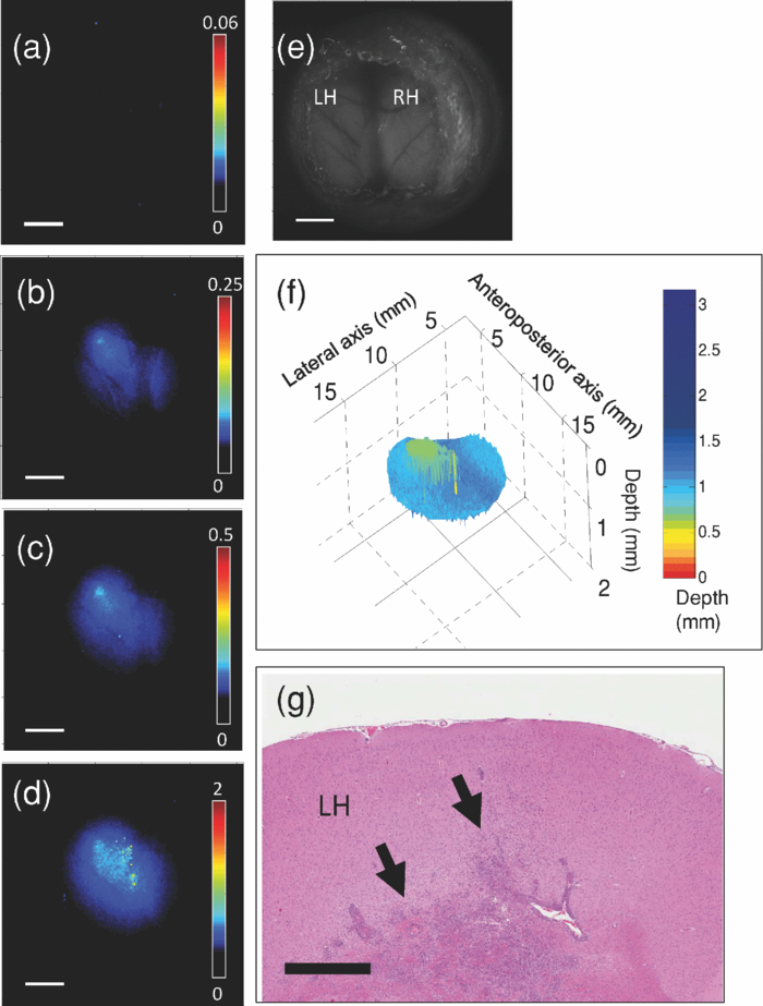

Fig. 5

Same as Fig. 4 for an animal in which the tumor was closer to the cortical surface.

It is useful to approximate tumor depth in the histology images so as to compare them to the depth-resolved fluorescence maps. In Fig. 4, the tumor is fully buried in the left hemisphere according to the depth-resolved fluorescence topography, ranging in depth from 0.65 to 1.8 mm, with a central tumor mass closest to the surface at 0.65 mm. The H&E-stained section indicates depths of 0.95–2 mm in the left hemisphere, with the central tumor mass closest to the surface at 0.95 mm. In Fig. 5, the depth-resolved topography indicates a large surface tumor located in the central region of the exposed left hemisphere and subsurface tumor ranging from 0 to 0.6 mm deep surrounding this central tumor mass. The H&E stain also indicates a tumor mass in the central region of the left hemisphere, with small, dispersed tumor inclusions through the left hemisphere ranging in depth from 0 to 1 mm. These discrepancies between the fluorescence depth estimations and tumor depth in H&E-stained slides may be partly explained by the significant difficulties in quantitative spatial analysis of histology slides, i.e., thin tissue 5 μm thick may stretch or tear, and formalin-fixed tissue is spatially distorted; however, the depth approximations from H&E stains provide a reasonable validation of the depth-resolved fluorescence technique in vivo.

5.

Discussion and Conclusion

These first studies illustrate the feasibility of this technique in phantoms and in a small-rodent brain tumor model, and show that one could expect to detect localized fluorescence up to ∼3 mm below normal brain surface using PpIX. This in itself may be very useful in guiding the final resection steps in glioma (or other intracranial tumor) patients to ascertain the presence and location of any noncontiguous tumor nests lying below the surface of the surgical resection bed. For this and other applications, it would also clearly be of value to map the tumor topography to greater depths. The restricted depth of subsurface imaging is a fundamental limitation of any fluorescence-based technique. One solution is to use fluorophores (including nanoparticle-based agents) with high quantum yield and/or excitation and emission in the red-to-NIR wavelength range (such as indocyanine green, although this dye has poor quantum yield). Such experiments are in progress. Note that this technique works well with PpIX because it has a large Stokes shift and a wide absorption (fluorescence excitation) band over which the tissue absorption varies significantly. For fluorophores with a small Stokes shift the available part of the fluorescence emission band is reduced due to the absorption-emission overlap, limiting the signal-to-noise ratio of the images. In the case of a narrow excitation spectrum, the effect will be to reduce the depth dynamic range over which imaging can be done.

With the geometry used in this work, diffusion theory typically has difficulty modeling the fluence rate near the surface and at low albedo. However, this is generally not a major limitation in this work. For example, using average brain tissue optical properties and at 0.5 mm beneath the surface, diffusion theory is within ∼20% agreement with Monte Carlo simulations for M ₁ (i.e., lowest albedo, poorest fit), 15% for M ₂ (second lowest albedo), and 10% for M ₃. The good accuracy under such extreme conditions (i.e., very low albedo and shallow depth) can be partly explained by the fact that diffusion theory overestimates the fluence rate, especially at shallow depths. By taking ratios for the M values, there is a degree of cancellation, resulting in a reduction of the error in calculating M ₁, M ₂, and M ₃.

Inaccuracies in the tissue optical properties will cause errors in the depth estimation. Variation in the tissue optical absorption is caused mainly by variations in blood perfusion (total hemoglobin concentration) and oxygen saturation. Hence, variations in μ_a at a given wavelength are in part coupled to that at other wavelengths in the visual-NIR region. For example, a ±25% variation in the nominal hemoglobin concentration ([Hb]) of 2 mg/mL induces about a ±10% uncertainty in the depth estimate at 2 mm. Depending then on the depth precision needed for effective surgical guidance, it may be necessary to measure the tissue optical properties to account for the dynamic changes during resection. This could be done using a supplementary device, such as our recently reported diffuse reflectance probe,¹⁹ or a spatially modulated imaging method that provides a diffuse optical tomographic reconstruction near the tissue surface.²²

It is of interest to ask how buried fluorescing objects with complex shapes may be resolved. If there are multiple sources of fluorescence (e.g., several separate nests of tumor at different depths) and lateral separations, then the topographic appearance will depend on whether or not the objects are fully separate or overlap laterally. Thus, for example, if there are two laterally overlapping objects at different depths, then the reconstructed surface will show the top surface layer of the nearest object contiguous with the top surface of the nonoverlapping part of the deeper object. Two nonlaterally overlapping objects, such as the separate tumors in the right and left hemispheres in Fig. 5, would appear as two distinct objects at different depths; however, there is a clearly complex interplay between the lateral and depth resolutions that needs further detailed investigation. Further studies using Monte Carlo models are planned to address this issue.

The concept of topographic imaging of subsurface fluorescent structures could be useful for a range of different applications beyond that demonstrated here, including, for example, determining subsurface blood vessels during surgery (using a vascular fluorophore), sentinel lymph node and lymph flow mapping with indocyanine green,^{23, 24} determining the depth of dermatological or other vascular lesions to help target laser therapies, nondestructive testing of nonbiological materials, and possibly for encryption and biosecurity.