
|
|
1.IntroductionKnowledge of refractive index distributions in biological samples can be used to quantify local nonaqueous density,1 image cell fluctuations,2 and study light scattering in tissue, which is relevant to deep tissue microscopy3 and applications of light scattering for disease diagnosis.4 In tomographic phase microscopy (TPM),5 the projection of a sample refractive index is imaged using a phase-shifting heterodyne interferometer6 with multiple directions of illumination. A filtered back-projection algorithm is then used to calculate a 3-D reconstruction of the sample refractive index. TPM is related to digital holographic microscopy (DHM),7, 8 which has also been used to measure tomographic images of cells. The major differences are: 1. in TPM the camera is at an image plane, whereas in DHM it is not and 2. in TPM the illumination angle in the sample remains fixed, while in DHM the illumination angle is fixed while the sample is rotated.9 Another related study used a propagation-based quantitative phase microscopy technique10 with sample rotation to generate tomographic images.11 The speed of tomographic imaging in TPM, DHM, and similar methods is limited by the requirement of acquiring a large number of 2-D phase images. In a DHM study of biological samples,9 acquiring data for a single tomogram required about 90 s. Similarly, a single TPM tomogram required about 10 s of data acquisition.5 Improving the speed of tomographic imaging will open up new possibilities for imaging rapidly changing, moving, or flowing cells. The acquisition time of TPM has been limited by two factors. First, for optimum image quality, phase images must be acquired at approximately 100 illumination angles; each phase image requires the capture of four raw frames for a total of 400 images per tomogram. Second, the galvanometer controlling sample illumination angle must be held constant during the acquisition of the four frames, requiring a settling time of approximately 100 ms after each change in angle. In this report, we describe an implementation of TPM using a spatial fringe pattern demodulation technique.12, 13 The method uses only 150 raw images per tomogram and does not require galvanometer settling time. As a result, full 3-D tomograms can be acquired at a rate of 30 Hz. 2.MethodsThe set up (Fig. 1) resembled the TPM system described previously5 without acousto-optic frequency shifting in the reference arm. A helium-neon laser beam (λ = 632.8 nm) was divided into sample and reference arm paths by a beamsplitter. In the sample arm, the beam was reflected from a galvanometer-mounted mirror (HS-15, Nutfield Technology, Hudson, New Hampshire). A lens (L1, f = 250 mm) was used to focus the beam at the back focal plane of an oil-immersion condenser lens (Nikon 1.4 NA), which recollimated the beam to a diameter of approximately 600 μm. Light passing through the sample was collected by an oil-immersion objective lens (Olympus UPLSAPO 100XO, 1.4 NA), and an achromatic doublet tube lens (f = 200 mm) was used to focus an image of the sample onto the camera with magnification M = 250. The reference laser beam was enlarged by a 10× beam expander (L2, L3) and combined with the sample beam through a beamsplitter. The resulting interference pattern was captured at 10-bit resolution by a high speed complementary metal oxide semiconductor (CMOS) camera [Photron (San Diego, California) Fastcam APX RS, 512×512 pixels]. A mercury arc lamp, LED illuminator, dichroic mirror, optical filters, and charge-coupled device (CCD) camera [Photometrics (Tuscon, Arizona) CoolSnap HQ] were also integrated into the setup for correlated bright-field and fluorescence imaging. The galvanometer was driven by a symmetric triangle wave with amplitude corresponding to ±60 deg at the sample and frequency of 15 Hz. A total of 150 images were acquired during each galvanometer sweep. Irradiances at the detector plane were ∼10 μW/cm2 for both the sample and reference fields; camera exposure times were typically ∼20 μs. Fig. 1Spatial modulation tomography setup. HeNe: helium-neon laser. In sample path (red): BS beamsplitter, GM galvanometer-controlled mirror, C condenser lens, θ beam tilt angle, S sample, OBJ objective lens, and DBS dichroic beamsplitter. In reference path (blue): BE beam expander. TL tube lenses, CMOS camera, and L1, L2, L3 lenses. CCD: camera for bright-field and fluorescence imaging (light path shown by dotted line). Not shown: illuminators and filters for bright-field and fluorescence imaging.  To obtain angle-dependent quantitative phase images, we used a fringe pattern demodulation technique.12, 13 First, we calculate the Fourier transform of the raw image; it contains peaks centered at 0 and [TeX:] $ \pm \vec q_\theta$ , where [TeX:] $\vec q_\theta$ is the spatial frequency of the fringe pattern equal to the difference between sample and reference wave vectors at the image plane. The Fourier components were then shifted by [TeX:] $ \vec q_\theta$ such that the [TeX:] $ + \vec q_\theta$ peak is translated to 0. A 2-D Hanning low-pass filter was applied to select only this central component. Applying the inverse Fourier transform then gave a complex-valued function [TeX:] $Z{}_\theta (x,y)$ , from which the phase image was calculated by [TeX:] $\phi _\theta (x,y) = {\rm arg}Z{}_\theta (x,y)$ . To achieve phase images with optimum spatial resolution, two conditions need to be met. First, the period of spatial fringes should be no larger than the diffraction-limited spot, which corresponds to approximately 0.3 μm at the sample. Second, for adequate sampling of the fringe, the pixel resolution should be fine enough to have at least three pixels per fringe; we found four pixels per fringe to be optimal. For our camera pixel size of 17 μm, we set the magnification to be 250 such that the four pixels correspond to 272 nm, satisfying both conditions. In the original TPM experiment,5 due to the rotation of the sample beam the fringe spatial frequency varied in magnitude from 0 to its maximum value [TeX:] $k\left| {\theta _{\max } } \right|/M$ , where k = 2π/λ. This large variation in spatial frequency impedes the maintenance of an optimal spatial frequency of the interference fringe. To avoid this problem, we introduced a fixed tilt of the reference beam in a direction normal to the sample beam tilt, with an angle such that in the absence of sample beam tilt there were four pixels per fringe in the y direction, as illustrated in Fig. 2. The fringe period is fixed along the y direction as the sample angle is varied from –θmax to + θmax [Figs. 2b, 2c, 2d). To calculate quantitative phase images, we applied the demodulation process only along the y direction. Fig. 2(a) Sample and reference beam geometry incident on image plane. k [TeX:] $_{R}$ : reference beam wave vector. k [TeX:] $_{S}$ (θ): sample beam wave vector. (b), (c), and (d) Detail of raw images of a 10 μm polystyrene bead for θ = −θmax, 0, and θmax. Scale bar: 5 μm. (e), (f), and (g) Corresponding phase images. Color bar, phase in radians.  A set of angle-dependent background phase images was acquired with no sample present and was subtracted from the sample phase images to reduce fixed-pattern noise from dust, optical aberrations, and imperfect optical alignment. We used the background-subtracted phase images to reconstruct the 3-D refractive index of the sample using a diffraction tomography algorithm based on the Rytov approximation, as reported earlier.14 This algorithm produces high resolution 3-D refractive index maps by accounting for the effects of diffraction in out-of-focus planes. It therefore yields images with extended depth of field, as described previously using a different strategy.15 Our algorithm gives the sample index relative to the surrounding medium; absolute index calibration was done using known values for the index of the culture medium.16 For cell imaging, cells were dissociated from culture dishes and allowed to attach to cover slips in normal culture medium [Mediatech (Vanassas, Virginia) DMEM + 10% fetal calf serum] for about 6 h at 37º C before imaging at room temperature. Coverslips were placed inside a flow chamber [custom made or Bioptechs (Butler, Pennsylvania) FCS2]. The culture medium was injected into the chamber using either a manual syringe or a syringe pump (Harvard Apparatus (Holliston, Massachusetts) PHD 22/2000). A valve was used to switch the input to the flow chamber to either a culture medium containing 0.5% acetic acid (for acetic acid experiments) or a hyperosmolar phosphate-buffered saline solution (for osmolarity experiments). Using the syringe pump, the hyperosmotic solution was injected into the chamber at a rate of 1.5 mL/min. We continuously acquired tomograms while the new medium was added. Data acquisition was performed using custom software written in MATLAB (MathWorks, Natick, Massachusetts) software. The 3-D diffraction tomography reconstruction algorithm was performed by custom software written in C. The rest of the data analysis was performed by custom software written in MATLAB. Using a computer running Windows XP 64-bit edition with a Intel Core 2 6600 processor running at 2.4 GHz and 2.93 GB of RAM, the computation time required to construct a single tomogram from 150 interferogram images was approximately 5 min. 3.ResultsAs in our previous study, we first validated our tomographic measurements using samples of 10-μm polystyrene beads [Polysciences (Warrington, Pennsylvania) 17136, n = 1.588 at λ = 632.8 nm] immersed in oil with a slightly smaller refractive index [Cargille (Cedar Grove, New Jersey) 18095, n = 1.559 at λ = 632.8 nm). We measured a refractive index difference Δn = 0.028 ± 0.001, in good agreement with the manufacturer's specifications. By analyzing the sharpness of the bead edge in tomograms, we estimated the spatial resolution to be 0.6 μm in the x-y plane and 0.75 μm in the z direction. To demonstrate the instrument's capabilities, we first monitored changes in the structure of a single cell during exposure to acetic acid. Acetic acid is widely used during colposcopy to identify suspicious sites on the cervix due to its whitening effect in precancerous lesions.17 Previously we showed that acetic acid causes an increase in refractive index inhomogeneity throughout a cell, and increases the index of the nucleolus.5 However, the time course of these changes was unclear due to a limited temporal resolution. To examine these changes in refractive index in detail, we acquired tomograms of a HeLa cell while the cell was exposed to a new medium containing acetic acid (see 1). Almost all changes in the cell structure were found to occur within a 2.75-s interval. Figures 3a, 3b, 3c show x-y slices through the center of the cell, at the start, midpoint, and end of this interval. An increase in refractive index heterogeneity is observed throughout the cell, and the index of the nucleolus increases dramatically. To assay the effects of acetic acid on different components in the cell, we partitioned the x-y slices into three distinct regions of interest (ROIs) as follows: 1. The region between the cell boundary and nuclear boundary, 2. The region enclosed by the nuclear boundary but not including the nucleolus, and 3. The nucleolus. Boundaries between ROIs [Fig. 3d] were drawn manually based on correlations between index tomograms, bright-field images, and widefield fluorescence images using the nucleic acid stain SYTO (Invitrogen, Carlsbad, California). Video 1Video of refractive index tomograms (cross section in x-y plane) of a HeLa cell during exposure to acetic acid solution, from Fig. 3. (QuickTime, 1.7 MB).  Figure 3e shows the time dependence of the average refractive index of the three ROIs. In the nucleolus (ROI 3), we observe a steady increase in average index, which reaches a stable value about 1.386 within about 2 sec. The remainder of the nucleus (ROI 2) exhibits an average index with similar time course but in the opposite direction, decreasing from about 1.364 to 1.359. As we reported previously,5 we find that the average refractive index of the nucleus, apart from nucleoli, is smaller than that of the cytoplasm. The time dependence of the average index in nucleus and nucleolus suggests a condensation of nuclear proteins into the nucleoli. The average refractive index of parts of the cell outside the nucleus (ROI 1) was largely unaffected by the addition of acetic acid. Optical scattering properties of a cell are largely determined by spatial variations in refractive index. To characterize these variations, we calculated the standard deviation σn of refractive index in the three ROIs [Fig. 3f] as a function of time. All three ROIs display a marked increase in refractive index heterogeneity. Remarkably, the three ROIs converge to similar large values for postacetic acid σn, despite a difference in preacetic acid values of about 40%. The more than two-fold greater increase in σn for the nucleus and nucleolus compared with the rest of the cell suggests that increased whitening of precancerous cells may reflect the greater nuclear-to-cytoplasmic volume ratio in such cells.18 Fig. 3Refractive index tomograms (cross section in x-y plane) of a HeLa cell during exposure to acetic acid solution at (a) t = 0.0 s, (b) t = 1.3 s, and (c) t = 2.6 s. Scale bar: 5 μm. Image sequence recorded at 30 fps. (d) Regions of interest (ROIs) described in text. (e) Average refractive index of each ROI. (f) Standard deviation σ [TeX:] $_{n}$ of refractive index for each ROI. Solid line: ROI 1. Dashed line: ROI 2. Dotted line: ROI 3. 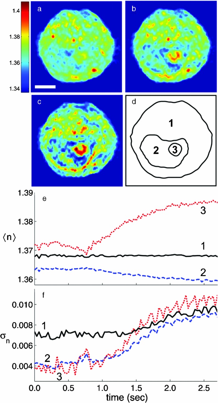 We performed a similar analysis to monitor changes in shape and structure of a single cell during exposure to a hypertonic buffered saline solution (see 2). Figure 4 shows an HT29 (human colonic adenocarcinoma) cell during a change in solution osmolarity from 300 to 975 mosm/L. To determine the changes in index of refraction of different components of the cell, a 2-D mask was drawn around a section of the cytoplasm, nucleolus, and nucleus regions. Because the boundary of the cytoplasm and other organelles varies slightly over the course of the video, the masks were drawn to maintain validity throughout the video. The average index of refraction inside each mask was calculated over the 15.4 s of recording time. After exposure to the hyperosmolar solution, the cell shrunk, and the average nuclear and cytoplasmic refractive indices exhibited a roughly linear increase of approximately 1.6 × 10⁻³/s and 1.7 × 10⁻³/s, respectively. The nucleolar refractive index increased only slightly. Fig. 4Refractive index tomograms (x-y slice) of an HT29 cell during exposure to hyperosmolar solution at time (a) 0.0 s, (b) 7.6 s, and (c) 15.4 s. (d) Time-dependent average refractive index of three regions of interest as described in text. 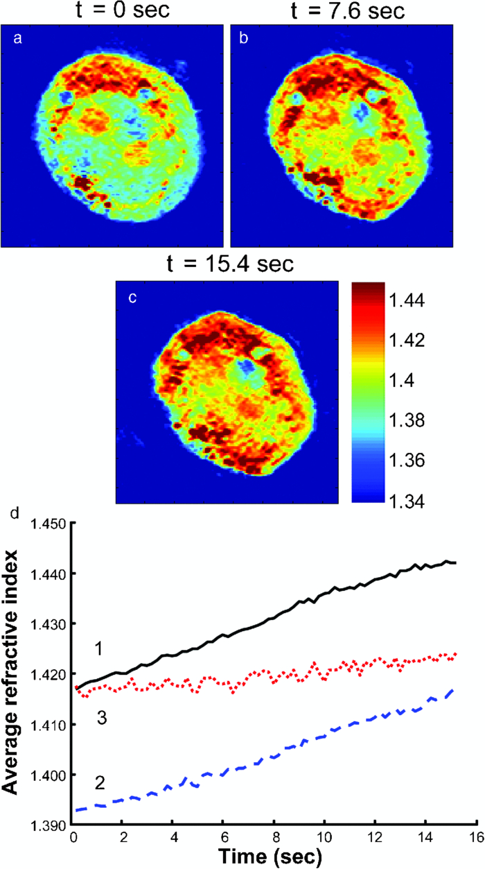 Video 2Videos of refractive index tomograms (x-y slice) of an HT29 cell during exposure to hyperosmolar solution, from Fig. 4. (QuickTime, 2.3 MB).  In summary, the use of spatial fringe pattern demodulation enables the acquisition of tomograms about 300 times faster than with the previous phase shifting technique. We use the improved system to measure region-specific temporal dynamics of refractive index on changes in acidity and osmolarity. Video-rate acquisition will also make it possible to acquire tomograms of flowing cells, with applications to studies of cell structure using flow cytometry or microfluidic chambers.16 AcknowledgmentsThis work was funded by the National Center for Research Resources of the National Institutes of Health (P41-RR02594-18), the National Science Foundation (DBI-0754339), and Hamamatsu Corporation. ReferencesR. Barer,
“Determination of dry mass, thickness, solid and water concentration in living cells,”
Nature, 172 1097
–1098
(1953). https://doi.org/10.1038/1721097a0 Google Scholar
Y. Park, M. Diez-Silva, G. Popescu, G. Lykotrafitis, W. Choi, M. S. Feld, and
S. Suresh,
“Refractive index maps and membrane dynamics of human red blood cells parasitized by Plasmodium falciparum,”
Proc. Natl. Acad. Sci. U S A, 105 13730
–13735
(2008). https://doi.org/10.1073/pnas.0806100105 Google Scholar
F. Helmchen, and
W. Denk,
“Deep tissue two-photon microscopy,”
Nat. Methods, 2 932
–940
(2005). https://doi.org/10.1038/nmeth818 Google Scholar
Handbook of Optical Biomedical Diagnostics, SPIE Press, Bellingham, UK
(2002). Google Scholar
W. Choi, C. Fang-Yen, K. Badizadegan, S. Oh, N. Lue, R. R. Dasari, and
M. S. Feld,
“Tomographic phase microscopy,”
Nat. Meth., 4 717
–719
(2007). https://doi.org/10.1038/nmeth1078 Google Scholar
C. Fang-Yen, S. Oh, Y. Park, W. Choi, S. Song, H. S. Seung, R. R. Dasari, and
M. S. Feld,
“Imaging voltage-dependent cell motions with heterodyne Mach-Zehnder phase microscopy,”
Opt. Lett., 32 1572
–1574
(2007). https://doi.org/10.1364/OL.32.001572 Google Scholar
F. Charriere, A. Marian, F. Montfort, J. Kuehn, T. Colomb, E. Cuche, P. Marquet, and
C. Depeursinge,
“Cell refractive index tomography by digital holographic microscopy,”
Opt. Lett., 31 178
–180
(2006). https://doi.org/10.1364/OL.31.000178 Google Scholar
M. Debailleul, B. Simon, V. Georges, O. Haeberle, and
V. Lauer,
“Holographic microscopy and diffractive microtomography of transparent samples,”
Meas. Sci. Technol., 19 074009
(2008). https://doi.org/10.1088/0957-0233/19/7/074009 Google Scholar
F. Charriere, N. Pavillon, T. Colomb, C. Depeursinge, T. J. Heger, E. A. D. Mitchell, P. Marquet, and
B. Rappaz,
“Living specimen tomography by digital holographic microscopy: morphometry of testate amoeba,”
Opt. Express, 14 7005
–7013
(2006). https://doi.org/10.1364/OE.14.007005 Google Scholar
D. Paganin and
K. A. Nugent,
“Noninterferometric Phase Imaging with Partially Coherent Light,”
Phys. Rev. Lett., 80 2586
(1998). https://doi.org/10.1103/PhysRevLett.80.2586 Google Scholar
A. Barty, K. A. Nugent, A. Roberts, and
D. Paganin,
“Quantitative phase tomography,”
Opt. Commun., 175 329
–336
(2000). https://doi.org/10.1016/S0030-4018(99)00726-9 Google Scholar
M. Takeda, H. Ina, and
S. Kobayashi,
“Fourier-transform method of fringe-pattern analysis for computer-based topography and interferometry,”
J. Opti. Soc. Am., 72 156
–160
(1982). https://doi.org/10.1364/JOSA.72.000156 Google Scholar
T. Ikeda, G. Popescu, R. R. Dasari, and
M. S. Feld,
“Hilbert phase microscopy for investigating fast dynamics in transparent systems,”
Opt. Lett., 30 1165
–1167
(2005). https://doi.org/10.1364/OL.30.001165 Google Scholar
Y. J. Sung, W. Choi, C. Fang-Yen, K. Badizadegan, R. R. Dasari, and
M. S. Feld,
“Optical diffraction tomography for high resolution live cell imaging,”
Opt. Express, 17 266
–277
(2009). https://doi.org/10.1364/OE.17.000266 Google Scholar
W. S. Choi, C. Fang-Yen, K. Badizadegan, R. R. Dasari, and
M. S. Feld,
“Extended depth of focus in tomographic phase microscopy using a propagation algorithm,”
Opt. Lett., 33 171
–173
(2008). https://doi.org/10.1364/OL.33.000171 Google Scholar
N. Lue, G. Popescu, T. Ikeda, R. Dasari, K. Badizadegan, and
M. Feld,
“Live cell refractometry using microfluidic devices,”
Opt. Lett., 31 2759
–2761
(2006). https://doi.org/10.1364/OL.31.002759 Google Scholar
E. Burghardt, H. Pickel, and
F. Girardi, Primary Care Colposcopy: Textbook and Atlas, Thieme Medical Publishers, New York
(2004). Google Scholar
D. C. Walker, B. H. Brown, A. D. Blackett, J. Tidy, and
R. H. Smallwood,
“A study of the morphological parameters of cervical squamous epithelium,”
Physiol. Measure., 24 121
–135
(2003). https://doi.org/10.1088/0967-3334/24/1/309 Google Scholar
|


