2.1.

Instrumentation

The UV-VIS DRS system, as depicted in Fig. 1(a), consists of a 450-W xenon lamp as the broadband light source (FL-1039, HORIBA Jobin Yvon, New Jersey), a laboratory-made self-calibration fiber optic probe to deliver illumination light to and collect diffusely reflected light from the tissue sample, and an imaging spectrometer with a 2-D charge-coupled decide (CCD) camera (iHR-320, HORIBA Jobin Yvon, New Jersey). The fiber optic probe has two channels: a tissue sensing channel (referred to as tissue CH) to collect a diffuse reflectance spectrum from a tissue sample, and a calibration channel (referred to as Cal CH) to collect a calibration spectrum concurrently with the tissue measurement, which can be used for real-time instrument and probe calibration. The probe uses a large core (400 μm) 1×2 fiber splitter (Fiber Optic Network Technology Company, British Columbia, Canada) as the source fiber for both sample illumination and self-calibration (the red fibers in Fig. 1). The light launched into the common arm of the splitter is divided into two channels, 80% to the tissue channel and 20% to the calibration channel. At the probe tip, eight 200-μm (core diameter) detection fibers (the blue fibers in Fig. 1) form a ring around the 400-μm tissue illumination fiber and collect the diffusely reflected light from the sample. The center-to-center distances between the single illumination fiber and the eight detection fibers range between 690 and 860 μm. The self-calibration illumination fiber terminates inside the rigid part of the probe tip, as shown in Fig. 1(b), and a portion of the calibration light is specularly reflected by the polished end surface of a stainless steel rod and coupled back into a 200-μm (core diameter) calibration return fiber (the green fiber in Fig. 1). Since the proximal ends of the calibration fibers and stainless steel rod are aligned and permanently fixed together inside a short piece of stainless steel capillary tube using epoxy, as shown in Fig. 1(b), the relative angles, distance, and spacing of the two fibers and the rod are all fixed. The reflector does not have to be a specular reflector, and any reflector can be used as long as it provides a comparable signal level as the tissue channel. All 200-μm fibers are made of identical silica/silica, high –OH optical fibers with numerical apertures (NA) of 0.22 (Polymicro Technologies, Phoenix, Arizona) to ensure the same bending response. This new probe design guarantees that the two channels respond to changes of the lamp emission intensity in the same manner.

Fig. 1

Schematic of (a) the UV-VIS DRS system with a splitter-based self-calibration fiber optic probe, and (b) the probe tip showing the termination of the fibers inside the probe housing. The detection fibers and calibration return fibers in the detection bundle are imaged onto the 2-D CCD as two separate tracks. (Color online only.)

In the detection fiber bundle, the detection fibers and the calibration return fiber are arranged into two columns, with two rows of dead fibers of the same diameter (the white fibers) for spacing between the two channels, as shown in Fig. 1(a). The fiber bundle is coupled to the imaging spectrograph iHR-320 via a reflective optics coupler with a 1:1.2 magnification. The collected diffuse reflectance and calibration beams are diffracted and projected onto different areas of the CCD camera and recorded by the laptop computer. The CCD chip has 1024 (horizontal) × 256 (vertical) pixels with a pixel size of 26 × 26 μm. The vertical axis is used to separate the self-calibration channel and the sensing channel, while the horizontal axis is used to detect the diffracted incident light. Because the spectrometer is optimized for spectroscopy (the CCD is in the tangential focal plane), relatively large spherical aberrations were measured in the vertical direction of the CCD. This means the image of an active fiber on the CCD in the vertical direction is larger than the diameter of the fiber. Therefore, two dead fibers were used to separate the two channels on the CCD, as indicated in Fig. 1(a). Pixels 62 to 92 along the vertical axis are binned for the self-calibration channel, while pixels 96 to 168 are binned for the sensing channel with three pixels left for spacing between the two channels, with no measurable cross talk on the CCD.

Each scan of the spectrometer covered only 128.7 nm. The input slit width of the spectrometer was set to 0.6 mm, resulting in a wavelength resolution of 1.4 nm. A complete spectrum from 350 to 600 nm took two scans with a low scan covering 349.4 to 479.8 nm and a high scan covering 472.2 to 600.9 nm. In addition to maintaining high wavelength resolution, acquiring two separate scans for the low and high wavelength ranges enabled the use of different integration times to achieve comparable signal for the entire wavelength range.

2.2.

Characterizing Different Sources of Systematic Errors

Three major sources of errors, including day-to-day variations in intensity, lamp warm-up, and fiber bending loss, were measured with the DRS system and SC probe B. First, day-to-day variations in lamp intensity were characterized under the same experimental conditions by taking five consecutive scans from the same Spectralon reflectance standard (Spectralon) after a lamp warm-up period of 60 min (to remove the effect of instrument warm-up drift as a variable) per day on each of two different days. The same experimental condition means that the instrument, probe-instrument interface, probe-Spectralon coupling, and fiber bending were unchanged between the two different days. Second, the effect of lamp warm-up was characterized by acquiring spectra from the same Spectralon using SC probe B at 13 time points between 2 and 60 min after the lamp was turn on for each of two off/on cycles. The intensity counts at two wavelengths of 475 and 575 nm were plotted against time to show lamp intensity fluctuations during warm-up (the intensity fluctuation after the warm-up period was provided in the lamp specifications from the vendor to be within 5%). Finally, after the lamp warm-up period, fiber bending loss was tested by wrapping the detection arm of the probe on a rod 2 and 3 cm in diameter (D), respectively for three turns each. Five consecutive scans were acquired from the Spectralon within a period of 5 min under each bending diameter (no bending, and D = 2 and 3 cm). The spectra for D = 2 and 3 cm were compared to the spectra obtained without fiber bending.

2.3.

Wavelength Response of the Calibration Channel

Although the two channels share the same light source and spectrometer, differences exist in the throughput between the two channels due to wavelength dependence of the splitter and coupling optics, and pixel-to-pixel variations in the CCD efficiency. This can be easily corrected by taking a one-time measurement on a spectrally flat diffuse reflectance standard, such as a Spectralon, and then generating a correction factor F _corr(λ) as defined in Eq. 1.

2.4.

Correction for Lamp Warm-Up

Of the three systematic errors characterized in Sec. 2.2, warm up introduced the greatest variation in source intensity. The capability of the DRS system for correction of system drift, which is dominated by the lamp intensity variations during warm-up, was evaluated. Specifically, reflectance and self-calibration spectra between 472 and 600 nm (high scan only) were collected from the Spectralon at different time points during instrument warm up. The probe tip was aligned perpendicular to the surface of the Spectralon at a fixed distance (∼1 mm) and maintained at that position throughout the experimental procedure. A calibrated reflectance spectrum was obtained by dividing the raw reflectance spectrum by the self-calibration spectrum collected simultaneously, and then was normalized to the calibrated first scan for variation calculation. The variation in the calibrated reflectance spectrum achieved with the new SC probe B was compared to that achieved with the original SC probe A described in our previous publication.²⁷

2.5.

Phantom Experiments

Tissue-simulating liquid phantoms were utilized to evaluate the performance of the DRS system for measuring tissue optical properties on two different days. The phantoms contained variable concentrations of hemoglobin (Hb) as the absorber and 1-μm polystyrene microspheres (07310-15, Polysciences, Incorporated, Warrington, Pennsylvania.) as the scatterer. Powder form of human Hb (H0267, Sigma-Aldrich Company, Saint Louis, Missouri) has been widely used as a stable absorber in optical spectroscopy by our group as well as by others.^{1, 28} The absorption coefficient (μ_a) was determined from a spectrophotometer measurement of a diluted Hb stock solution, and the reduced scattering coefficients ( [TeX:] $\mu_s^{\prime}$ ${\mu }_s^{\prime }$ ) was calculated using the Mie theory²⁹ for known size, density, and refractive index of the scatterers.

Two sets of phantoms with identical [TeX:] $\mu_s^{\prime}$ ${\mu }_s^{\prime }$ were obtained through 17 successive titrations of Hb from 1 to 31.9 μM for day 1 and 0.9 to 29.7 for day 2. Table 1 summarizes the Hb concentrations and expected phantom optical properties averaged over the wavelength range of 450 to 600 nm. Although the number of scatterers was fixed, the wavelength averaged [TeX:] $\mu_s^{\prime}$ ${\mu }_s^{\prime }$ decreased from 17.3 to 12.5 with successive dilution. The overall μ_a ranges from 0.016 to 4.65 cm⁻¹ for day 1 and 0.011 to 4.38 cm⁻¹ for day 2, over 450 to 600 nm.

Fig. 8

Extracted versus expected: (a) Hb concentrations and (b) wavelength-averaged reduced scattering coefficients from across-day data analysis, in which phantom 11 from a different day was used as a reference.

Table 1

Summary of the Hb concentrations and expected phantom optical properties averaged over the wavelength from 450 to 600 nm. Phantom 11 was selected as the reference phantom for all MC inversions.

A diffuse reflectance spectrum was measured with a calibration spectrum concurrently from each phantom using the SC probe B. On day 1, the measurements were taken 30 min after the instrument was turned on to eliminate the effect of source intensity variations due to instrument warm-up. On day 2, the measurements started only 2 min after the instrument was turned on to include the effect of source intensity variations due to instrument warm-up. On both days, a reflectance spectrum was also measured from the Spectralon immediately after all the phantom measurements using the same integration times as for the phantom measurements. Approximately 45 to 60 min elapsed between the first phantom and the Spectralon measurements on both days.

2.6.

Data Analysis

The data analysis procedures for tissue optical spectroscopy are outlined in Fig. 2. In this study, tissue-simulating liquid phantoms were used rather than tissue as the target, and one of the phantoms from the tissue-simulating phantom set was selected as the reference. Hemoglobin, in its oxidized form, was the only absorber in all phantoms.

Fig. 2

Data analysis procedures: (a) with Spectralon calibration and (b) with self-calibration.

The first step of the data analysis was calibration, which was performed using two approaches: Spectralon calibration and self-calibration, according to the procedures outlined in Fig. 2. With Spectralon-based calibration, the calibrated spectrum was obtained by dividing the reflectance spectrum (low or high scans) by the corresponding Spectralon measurement (the low or high scans with identical integration time). With self-calibration, the calibrated spectrum was obtained by dividing the reflectance spectrum by the self-calibration spectrum collected concurrently, and then by the correction factor. In both calibration approaches, a complete calibrated spectrum was assembled by scaling the calibrated low scan to the high scan at 476 nm (the middle wavelength of overlap between the two scans), and then splicing them into a single spectrum.

Next, the calibrated target tissue phantom spectrum was further normalized to a similarly calibrated reference phantom spectrum prior to analysis by a fast, scalable inverse MC model developed by our group to extract the tissue optical properties.¹ In this study, phantom 11 was selected as the reference phantom based on a previously published study by our group.²⁸ The calibration of the target tissue phantom spectrum against a reference phantom is needed to scale the MC modeled data to the experimentally measured data, while the calibration of the tissue and reference phantom spectra to the Spectralon or SC spectrum is carried out to account for day-to-day or real-time variations in system throughput, respectively.

The inverse MC model of reflectance that was used for extraction of the phantom optical properties consists of a forward model and an inverse model. In the forward model, a set of absorbers are presumed to be present in the medium, and the scatterer is assumed to be single sized, spherically shaped, and uniformly distributed. The wavelength-dependent absorption coefficients of the medium are calculated from the concentration of each absorber and the corresponding wavelength-dependent extinction coefficients. The wavelength-dependent [TeX:] $\mu_s^{\prime}$ ${\mu }_s^{\prime }$ is calculated from scatterer size, density, and the refractive index of the scatterer and surrounding medium from the Mie theory for spherical particles using freely available software.³⁰ The absorption and scattering coefficients are then input into the scalable MC physical model of light transport to obtain a modeled diffuse reflectance spectrum. In the inverse model, the modeled diffuse reflectance is adaptively fitted to the measured tissue diffuse reflectance. When the sum of squares error between the modeled and measured diffuse reflectance is minimized, the concentrations of absorber, scatter size, and density are extracted. An attribute of the scalable MC model of reflectance is that it accounts for the specific probe geometry used for diffuse reflectance measurements. A detailed description of this physical model is provided elsewhere.¹

Inversions were performed in the wavelength range of 450 to 600 nm for best signal-to-noise ratio. Two different approached were used: within-day data analysis, in which the target and reference phantoms were from same-day measurements, and across-day data analysis, in which the target and reference phantoms were from different days. The within-day analysis compares the accuracy of the two calibration approaches with and without lamp warm-up, while the across-day analysis tests the capability of the self-calibration to correct for day-to-day instrument drift (a larger drift was created by starting phantom measurements during lamp warm-up on day 2), and is representative of what would happen in an actual clinical setting.

3.1.

Sources of Systematic Errors

Figure 3(a) shows ten reflectance spectra from 470 to 600 nm (high scan only) collected from the same Spectralon on two different days with the experimental setup unchanged. The five consecutive scans on each day (in a single color or solid line) showed very small variations (less than 1%). Although the spectra from the two different days have similar line shape, the lamp intensity drift from day 1 to day 2 ranges from 3 to 7% over the entire wavelength range. This day-to-day lamp intensity fluctuation makes it necessary to have a reproducible calibration measurement before or after every clinical study, which usually takes 5 to 20 min of valuable time in a clinical setting. Figure 3(b) shows the lamp intensity at two wavelengths, 475 and 575 nm (normalized to the maximum intensity for 575 nm), over a period of 60 min after the lamp was switched on for two off/on cycles. An increase of 55% at 575 nm and 38% at 475 nm in the lamp intensity was observed in the first 30 min for the first cycle. The increases for the second cycle are 38% at 575 nm and 24% 475 nm. The intensity fluctuation was less than 5% between 30 and 60 min, which agrees with the lamp specification provided by the vendor. The source intensity variations are large, as shown in Fig. 3(b), due to the rapid increase in the lamp intensity at the early time points. The difference in the intensity change at the two wavelengths in the first 30 min also indicates that the line shape of the lamp spectrum changes over time during warm up and thus cannot be accounted for with a simple one-time calibration measurement. This source of error is currently accounted for by allowing the instrument to warm up for a certain period of time (30 min) prior to initiating the spectroscopic measurements. However, this assumes that the warm-up period stays the same each time, which may not always be a reasonable assumption. Figure 3(c) shows three sets of spectra (five in each color or solid line) that were collected between 470 and 600 nm (high scan only) for the case where there was no bending, a bending diameter of D = 3, and a bending diameter of 2 cm, respectively. Obviously, the bending-induced attenuation is significantly higher than the repeated measurements or day-to-day variations. An average fiber bending loss of 8.7 and 68.9% was observed at 470 nm for D = 3 and 2 cm, respectively. The sharp increase in the bending loss at D = 2 cm indicates that there was a significant increase in wave coupling from the guided modes to cladding (leaky) modes in the fibers. There is, to the best of our knowledge, no existing technology to correct for bending loss that occurs during a tissue or phantom measurement.

Fig. 3

Sources of instrumental errors. (a) Day-to-day lamp intensity fluctuations measured with SC probe B. Each color represents five consecutive scans per day from each of two days. (b) Lamp intensity fluctuations during a 60-min warm-up period normalized to the maximum intensity at 575 nm. (c) Intensity attenuation induced by fiber bending loss measured with SC probe B. Each color represents five consecutive scans under the same bending diameter. All of these measurements were made on a Spectralon reflectance standard with high scan only. (Color online only.)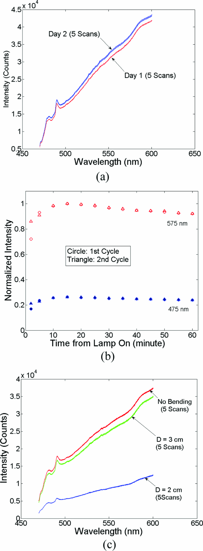

3.2.

Correction Factor

Figure 4(a) shows the raw reflectance spectrum from a Spectralon and the self-calibration spectrum collected concurrently after 30 min of lamp warm-up. The SC channel has a different wavelength response compared with the tissue channel, due to the use of a stainless-steel reflective rod and the free-space coupling from the calibration source fiber to the return fiber, as illustrated in Fig. 1(b). Thus a correction factor for this wavelength-dependent response was generated [defined in Eq. 1] for this particular probe and is shown in Fig. 4(b). The relatively large fluctuations between 450 and 500 nm of the correction factor could be due to multiple emission peaks in the lamp spectrum and the optical aberrations in the spectrometer, which might result in different wavelength scales for the two channels. It could also be caused by the splicing of the two scans that is required to cover a wavelength range from 350 to 600 nm using this instrument. However, the fluctuations should not affect the accuracy of the calibration as long as it is repeatable. The repeatability of the correction factor was measured by reattaching (10 times) the probe to the instrument, which may be required for probe sterilization, and the coefficient of variation (COV) was plotted in Fig. 4(c). The COV averaged over the wavelength range of 350 to 600 nm is 1.35%. The largest variation appears at the wavelength below 450 nm due to relatively low lamp intensity. In this work, spectral analysis of the phantom data was performed between 450 and 600 nm. The variation is mainly due to the probe adaptor design, which uses a setscrew to lock the collection fiber bundle into a tube on the instrument side and can be further reduced by alternate designs. The correction factor was saved in the computer and was used for subsequent calibrations using the procedures shown in Fig. 2(b). Each instrument and probe combination has its own wavelength-dependent response and requires a unique correction factor F _corr(λ). Using SC probe B with the correction factor, the sources of errors presented in Figs. 3(a), 3(b), and 3(c) can be corrected in real-time.

Fig. 4

Correction for wavelength dependence of the self-calibration channel between 350 and 600 nm (obtained from two scans): (a) raw spectra; (b) correction factor F _corr(λ); and (c) coefficient of variation of F _corr(λ) in 10 repeated experiments.

3.3.

Correction for Lamp Intensity Fluctuations

Figure 5(a) shows the raw reflectance spectra (high scans only) that were collected by SC probe B from the Spectralon at successive time points starting 2 min from when the lamp was turned on. The lamp intensity increased by 14 to 20% from 2 to 40 min, which is slightly lower than that measured in Fig. 3(b). What needs to be mentioned is that the spectra in Figs. 3(a), 3(c), and 5(a) were collected in three independent experiments, in which probe-to-Spectralon coupling and fiber bending were not repeatable. Therefore, the spectral intensities varied significantly among the three experiments. The dips around 542.5 nm in Fig. 5(a) could be due to a bad pixel on the CCD chip or a tiny crack in one of the collection fibers. Figure 5(b) shows the raw reflectance spectra divided by the calibration spectra collected concurrently and then normalized to the first scan. Dividing the raw spectra by the calibration spectra reduced the intensity fluctuations down to ±1% (except for the edge pixels, which were discarded during the splicing), demonstrating that the lamp fluctuations shown in Fig. 3(b) can be corrected by self-calibration. This also indicates that the repeatability of the correction factor is within ±1%. As a comparison, Figs. 5(c) and 5(d) show the raw and normalized self-calibrated reflectance spectra obtained using the SC probe A (with separate illumination fibers for tissue and calibration channels) at successive time points starting 5 min from when the lamp was turned on. Even with smaller lamp drifts (∼8%, resulting from the slightly longer warm-up time for the first measurement), the calibrated spectra still show a 4% variation, which is likely due to variation of the spatial distribution of the lamp emission during warm up.

Fig. 5

Correction for lamp intensity variations: (a) raw spectra from the Spectralon at various time points after the lamp was turned on, and (b) ratio between the Spectralon and self-calibration spectra normalized to the first scan using SC probe B. (c) Raw spectra from the Spectralon at various time points after the lamp was turned on, and (d) ratio between the Spectralon and self-calibration spectra normalized to the first scan using SC probe A.

3.4.

Phantom Experimental Results

The Spectralon- and self-calibrated reflectance spectra measured from phantoms 1 (lightest), 9 (medium), and 17 (darkest), all from day 1, are plotted over the full wavelength range from 350 to 600 nm in Fig. 6. The three intensity valleys at 415, 540, and 575 nm in all spectra correspond to the Soret band (400 to 450 nm), α band (540 nm), and β band (569 nm) of oxygenated hemoglobin, respectively. The absorption of the α and β bands in phantom 1 are hardly noticeable due to the low Hb concentration in this phantom. The self-calibrated and Spectralon calibrated spectra for phantoms 9 and 17 show excellent overlap. The small but distinct difference between the two calibrated spectra for phantom 1 is likely caused by instrument drift during the time elapsed (> 45 min) between the first phantom measurement and Spectralon measurement that was performed right after phantom 17.

Fig. 6

Spectralon- and self-calibrated phantom spectra for phantoms 1, 9, and 17, all from day 1.

3.4.1.

Within-day data analysis

In the within-day data analysis, the MC inversions were performed between the wavelengths of 450 and 600 nm for all target phantom spectra and reference phantom (phantom 11) from the same day. The extracted versus expected Hb concentrations and wavelength-averaged reduced scattering coefficients over 450 to 600 nm are plotted in Figs. 7(a) and 7(b), respectively. On either day, both the self- and Spectralon-calibration methods resulted in excellent agreement for the extracted and expected Hb concentrations (overall error within 8.8%) as well as for the reduced scattering coefficients (overall error within 4.5%). On day 2, in which phantom measurements were made during the lamp warm-up period, however, the extracted reduced scattering coefficients with the Spectralon calibration diverged considerably from the expected values at higher [TeX:] $\mu_s^{\prime}$ ${\mu }_s^{\prime }$ , which corresponds to the first few phantoms, and the overall error is higher than the other three sets shown in Fig. 7(b). This is due to the fact that Spectralon calibration, which was performed after the phantom studies, did not account for the variations in source intensity due to lamp warm up.

Fig. 7

Extracted versus expected: (a) Hb concentrations and (b) wavelength-averaged reduced scattering coefficients over 450 to 600 nm from within-day data analysis, in which phantom 11 from the same day was used as a reference.