

|
|
1.IntroductionIn two-dimensional (2-D) camera-based optical brain imaging either on an exposed neo-cortex or through a thinned skull, a collimated beam (often in the visible spectrum) incident onto the brain surface propagates inside the tissue. Depending on the optical properties being imaged (absorption or fluorescence), the optical imaging system collects either diffusely reflected or fluorescent light from the brain, forming 2-D images. Here, we disregard the effects of scattering changes because they are negligible in the visible spectrum. Both absorption [such as with intrinsic optical imaging (IOI), which images the absorption of the hemoglobin] and fluorescence imaging [such as with voltage-sensitive dye imaging (VSDI)] have been used widely to map neo-cortical functions in vivo.1, 2, 3, 4, 5, 6 For example, local blood oxygenation and total hemoglobin concentration often change with neuronal activity in the cortical tissue, leading to a change in the absorption of incident light, and therefore, a difference in diffusely reflected light.3, 5, 6 Hence, images formed by reflected light can reveal cortical function. On the other hand, fluorescence imaging may reveal different aspects of neuronal activity depending on the dyes employed. For example, voltage-sensitive dyes reflect the electric activities of neurons. Both approaches have been used extensively in studying the functional maps and spatiotemporal dynamics of the neuronal activity of the somatosensory, visual, and auditory cortexes, as well as the olfactory bulbs in animal models such as mice, rats, cats, and monkeys.3, 4, 5, 6, 7, 8 Tissues at different depths of the cortex contribute to the image on the camera [i.e., the measured signal (the intensity of each pixel of the image) is a weighted sum of the real signal from these tissues]. We use the term “depth sensitivity” to describe this weighting function. Because of light scattering in the cortex, even a single point in the brain tissue will not result in an image consisting of a diffraction-limited spot but a much larger region. The size of this region is determined not only by the configuration of the optical imaging system [numerical aperture (NA) and focal plane depth] but also by the optical properties of the tissue (such as the scattering and absorption coefficients). We use the term “spatial resolution” to characterize the size of this region due to an array of points throughout the cortical tissue. In general, both the spatial resolution and depth sensitivity may depend on the optical configuration of the imaging system. Hence, in order to optimize the imaging system and better interpret the experimental data and compare the results among different functional imaging modalities (including IOI, fluorescence imaging, and nonoptical-based approaches, such as functional magnetic resonance imaging), we need to characterize the spatial resolution and depth sensitivity as a function of NA and focal plane depth. The light scattering and absorption in biological tissues make it difficult to do so; however, Polimeni. have estimated the spatial resolution of IOI for a specific optical configuration using Monte Carlo simulation with tissue parameters describing the mammalian cortex.9 Their result of 240 μm is consistent with the experimental result of Orbach and Cohen.10 Other authors have mentioned a much smaller spatial resolution, though without offering evidence to support it.3 In summary, spatial resolution has been reported for only a few specific optical configurations and there is a lack of information for depth sensitivity. Propagation of light in a highly scattering medium such as the cortex is complicated and therefore, difficult to model by directly solving Maxwell equations. On the other hand, both absorption and fluorescence imaging, where the polarization and interference effects can be ignored, can be rigorously modeled with the radiative transfer equation (RTE). The analytical solution of RTE is known for only a limited number of simple experimental configurations, however, and it fails when we need to study light propagation near the boundaries or the light sources, as is the case for many 2-D optical brain imaging experiments. Monte Carlo simulation traces the trajectories of individual photons and offers a flexible yet rigorous approach to photon transport in highly scattering tissues. Since Wilson and Adam first introduced Monte Carlo simulation into the field of laser tissue interactions, it has been widely used to simulate light transport in tissues.11, 12, 13, 14 We have employed Monte Carlo simulation to calculate the spatial resolution and depth sensitivity of both the absorption- and fluorescence-based 2-D optical imaging under optical configurations typically encountered in camera-based optical brain imaging on the neo-cortex. In Sec.2, we present physical models of the problem and describe our method to reduce the number of Monte Carlo simulations to improve the efficiency of our calculation. Here, we have employed the RTE under the first Born approximation. This enables us to perform the Monte Carlo simulations using homogeneous tissue configuration and thus greatly reduce computational time. In Sec. 3, we show numerical results for spatial resolution and depth sensitivity under various combinations of NA and focal plane depth. In Sec. 4, we discuss the application of our results in optical brain-imaging experiments in vivo, especially, how to optimize NA and focal plane depth differently to satisfy different requirements of spatial resolution, depth sensitivity, and signal level. 2.MethodsFigure 1 illustrates the 2-D camera-based optical imaging system. A collimated light beam perpendicularly illuminates the brain tissue. For absorption imaging, diffusedly reflected light (marked by arrows) is collected by lens L1 and imaged onto a camera by lens L2.15 When there is no functional activation, the brain tissue scatters and absorbs light with homogeneous refractive index n 0, the anisotropic factor g 0, scattering, and absorption coefficients, μs0 and μa0, respectively; thus, the image on the detector plane is uniform. When a certain cortical region is functionally activated, its local optical properties, such as the absorption coefficient, will often be altered. Such spatial disturbance of the otherwise homogeneous optical property will lead to a small perturbation in the image on the detector, resulting in a nonuniform image. Therefore, in a typical functional imaging experiment, images are recorded both during and before the functional activation and the difference image is obtained as δI. For fluorescence imaging, fluorescence is imaged, instead of reflected light, by inserting a bandpass filter (BPF) in front of the detector. Thus, the difference image would reflect changes in local optical properties, such as the absorption coefficient and/or the fluorescent quantum efficiency η0. Ideally, this difference image would reflect the local variation of the optical properties at a particular depth inside the tissue, which, in turn, would represent the functional activation pattern of the tissue. As stated in the Introduction, due to both the scattering nature of cortical tissue and the limitations of the imaging system, this difference image is a “blurred” representation of the spatial disturbance of the local optical properties throughout the cortical depth. In fact, in 2-D optical imaging experiments, we do not have enough information to reconstruct the complete 3-D variation of the local optical properties from the difference images. Nevertheless, these difference images offer valuable information as to the spatial extent and magnitude of the functional activation provided that we understand the spatial resolution and depth sensitivity of the 2-D optical imaging method, which we will define and calculate for both absorption and fluorescence imaging. Fig. 1Schematic diagram of a camera-based optical imaging system. A collimated light beam illuminates the brain tissue. For absorption imaging, the backscattered light (marked by arrows) is collected by lens L1 and imaged onto a two dimensional detector plane by lens L2. For fluorescence imaging, a BPF is inserted in front of the camera allowing the detection of the fluorescence. The system is arranged in a 4f configuration. f: focal length of L1 and L2. BS: beamsplitter. NA: numerical aperture.  Figure 1 illustrates a “4f configuration” where the two lenses have the same focal length f and the same distances between the consecutive planes. To be precise the distances between the front focal plane of L1, L1, the back focal plane of L1 (the same as the front focal plane of L2), L2, the back focal plane of L2 (the same as the detector plane) are all f. Hence, the front focal plane of L1 in an optically clear medium is imaged directly onto the detector with a magnification M = 1. Because of its simplicity and wide application, we will mainly consider the 4f configuration in this paper.15 The potential deviation of our results from those of different configurations will be addressed briefly in Sec. 4. In many functional imaging experiments, the optical system can be varied by either changing the NA of L1 or placing different depths of the cortical tissue at the front focal plane of L1, as shown in Fig. 1. We will discuss the influence of these changes on spatial resolution and depth sensitivity. In order to define the spatial resolution for absorption imaging in the cortex, which often has columnar organization, we consider a single array of point absorbers along the optical axis and evenly distributed throughout the cortical depth [Fig. 2a]. Each point absorber acts as a local perturbation and results in a difference image with circular symmetry [Fig. 3a]. The summation of these images is then detected by the camera [Fig. 3b]. The spatial resolution can be defined as the full width at half maximum (FWHM) of that profile [Fig. 3c]. As displayed here, the spatial resolution indicates the minimal separation between two neighboring functionally activated columns that can be spatially resolved by the imaging system. To define the depth sensitivity, we consider multiple arrays of point absorbers evenly distributed throughout the cortical depth and with a cross-sectional area of L 2, where L is the lateral size of the functionally activated region inside the tissue [Fig. 2b]. These arrays of point absorbers act as the local perturbation. Because the point absorbers at all depths contribute to the difference image, the total intensity variation at one location (or pixel) on the detector δI(x d, y d) is the summation of all the individual intensity variation, δI z(x d, y d), where z indicates the depth [Figs. 4a and 4b]. Therefore, we define depth sensitivity as the ratio of the contribution from an individual depth z to the total contribution from all depths, i.e., δI z/δI [Fig. 4c]. Similarly, we can define spatial resolution and depth sensitivity for fluorescence imaging by replacing the absorbers with fluorescent targets inside the tissue. Both spatial resolution and depth sensitivity play important roles in accurately interpreting the data and in comparing data obtained using different imaging modalities and across species. Fig. 2Distributions of point disturbance in the absorption and fluorescence imaging. Absorption imaging: (a) A single array of point absorbers evenly distributed throughout the cortical depth (0–1 mm) and along the optical axis. (b) Multiple arrays of point absorbers evenly distributed throughout the cortical depth (0–1 mm) and with a lateral size of L. Fluorescence imaging: the distribution of a single array and multiple arrays of fluorescent targets are shown in (a, b), respectively. Their normalized staining profile can be either uniform (c) or nonuniform (d).  Fig. 3Definition of the spatial resolution. For absorption imaging: (a) The difference images due to individual point absorbers depicted in Fig. 2(a). (b) The summation of all these images. (c) The profile of the summed image along the radial direction. The spatial resolution is defined as the FWHM of this profile. For fluorescence imaging, the spatial resolution is defined similarly except that fluorescence targets replace point absorbers. 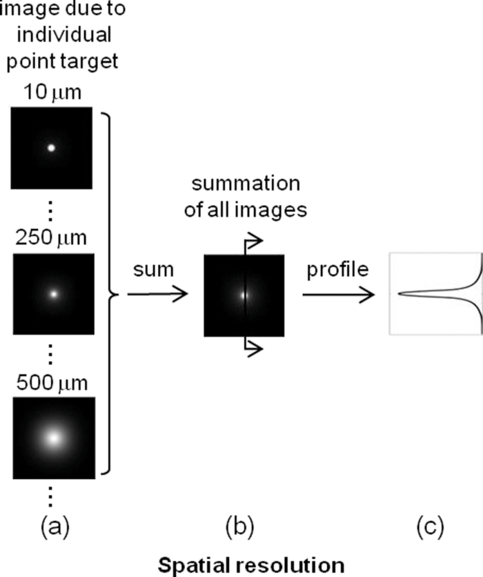 Fig. 4Definition of the depth sensitivity at the center of the detector. For absorption imaging, multiple arrays of point absorbers depicted in Fig. 2(b) are considered. The horizontal size of the array is L. (a) The contribution to the total intensity variation at the center of the detector from an individual layer of point absorbers at depth z is equivalent to the cropped image due to an individual point target at (0, 0, z) inside the tissue. (b) The total intensity variation at the center of the detector induced by all point absorbers within a certain depth is the summation over the area L 2 of the cropped image and depth. (c) The depth sensitivity is defined as the ratio of the contribution from an individual depth and the total contribution from all depths. The depth sensitivity of fluorescence imaging can be defined similarly except that fluorescence targets are used instead of point absorbers.  As can be seen, we need to know the corresponding difference images for absorption and fluorescence imaging, respectively, in order to calculate the spatial resolution and depth sensitivity. This requires an understanding of light propagation in a highly scattering medium, such as the cortex. As discussed earlier, the RTE provides an accurate description of this problem. However, there is no analytical solution to the transport equation in the situation of 2-D optical imaging, where we are interested in light propagating from near to within a few scattering lengths from the surface. Fortunately, in a typical functional imaging experiment, the local perturbation to the optical properties is relatively weak: only a few percent of that of the background. Hence, we can simplify the problem by using the first Born approximation to the RTE followed by Monte Carlo simulations. Below we will discuss the cases for absorption imaging and for fluorescence imaging. 2.1.Absorption imagingThe total absorption coefficient can be written as a sum of a homogeneous background component μa0 and a spatially varying perturbation δμa0(r), thus, μa(r) = μa0 + δμa(r). As discussed above, we use the first Born approximation to the RTE and express the perturbed radiance [TeX:] $\delta I(r_{\rm d}, \hat \Omega _{\rm d})$ , the intensity flowing in direction [TeX:] $\hat \Omega _{\rm d}$ and arriving at position r d on the detector plane, as follows: Eq. 1[TeX:] \documentclass[12pt]{minimal}\begin{document}\begin{equation} \delta I(r_{\rm d}, \hat \Omega _{\rm d}) = - \int\!\!\int\delta\mu_{\rm a}(r)I_0(r,\hat \Omega)G(r_{\rm d}, \hat \Omega _{\rm d} |r,\hat \Omega)d\hat \Omega d^3 r, \end{equation}\end{document}Eq. 2[TeX:] \documentclass[12pt]{minimal}\begin{document}\begin{equation} I(r) = \int {I(} r,\hat \Omega)d\hat \Omega . \end{equation}\end{document}Eq. 3[TeX:] \documentclass[12pt]{minimal}\begin{document}\begin{equation} \delta I(r_{\rm d}) = - \int\!\!\int\delta\mu_{\rm a}(r)I_0(r,\hat \Omega)G(r_{\rm d} |r,\hat \Omega)d\hat \Omega d^3 r. \end{equation}\end{document}2.1.1.Spatial resolutionTo calculate the spatial resolution, we consider a single array of point absorbers evenly distributed throughout the cortical depth and with an absorption coefficient of μa0 + Δμa0, where Δμa0 is the extra absorption due to the functional activation; thus, Eq. 4[TeX:] \documentclass[12pt]{minimal}\begin{document}\begin{equation} \delta \mu _{\rm a} (r) = \sum\limits_{0 \le z{}_i \le 1\,{\rm mm}} {\Delta \mu _{{\rm a}0} \delta (x,y,z - z_i)}, \end{equation}\end{document}Eq. 5[TeX:] \documentclass[12pt]{minimal}\begin{document}\begin{equation} \delta I(r_{\rm d}) = - \Delta \mu _{{\rm a0}} \sum\limits_{0 \le z \le 1\,\,{\mathop{\rm mm}\nolimits} } {\int {I_0 (z,\hat \Omega)G(r_{\rm d} |0,0,z,\hat \Omega)d\hat \Omega } } . \end{equation}\end{document}Fig. 5(a) A point absorber at (0, 0, z) in the absorption imaging acts as a negative light source that has an anistropic radiance – [TeX:] $I_0 (z,\hat \Omega)$ in the direction of [TeX:] $\hat \Omega$ . (b) A fluorescent target at (0, 0, z) in the fluorescence imaging acts as an isotropic light source with an intensity of I 0(z).  We employ Monte Carlo simulation to calculate both [TeX:] $I_0 (z,\hat \Omega)$ and [TeX:] $G(r_{\rm d} |0,0,z,\hat \Omega)$ using the homogenous optical properties μs0, μa0, n0, and g 0. We need one Monte Carlo simulation for [TeX:] $I_0 (z,\hat \Omega)$ , however, 100 different simulations for [TeX:] $G(r_d |0,0,z,\hat \Omega)$ , one for each point absorber located at a different depth z. Because Monte Carlo simulation is time consuming, it would be advantageous to reduce the number of calculations. To this end, we take advantage of the translational invariance of the tissue, the principle of reciprocity, and the 4f configuration to further simplify Eq. 5 into Eq. 6[TeX:] \documentclass[12pt]{minimal}\begin{document}\begin{eqnarray} \hspace*{-2pc}\delta I(x_{\rm d}, y_{\rm d}, z_{\rm d}) &=& - \Delta \mu _{a0} \sum\limits_{0 \le z \le 1\,{\rm mm}}\nonumber \\ && \hspace*{-.0pc}\times {\int\!\! {I_0 (z,\hat \Omega)G(x_{\rm d}, y_{\rm d}, z, - \hat \Omega |0,0,z_{\rm d})d\hat \Omega } } \end{eqnarray}\end{document}2.1.2.Depth sensitivityHere, we consider multiple arrays of point absorbers evenly distributed throughout the cortical depth (0–1 mm) and with a cross-sectional area of L 2 [Fig. 2b], thus, Eq. 7[TeX:] \documentclass[12pt]{minimal}\begin{document}\begin{equation} \delta \mu _{\rm a} (r) = \sum\limits_{\scriptstyle - L/2 \le x_i \le L/2 \hfill \atop {\scriptstyle - L/2 \le y_j \le L/2 \hfill \atop \scriptstyle 0 \le z_k \le 1\,\,{\rm mm} \hfill}} \Delta \mu _{{\rm a}0} \delta (x - x_i, y - y_j, z - z_k). \end{equation}\end{document}Eq. 8[TeX:] \documentclass[12pt]{minimal}\begin{document}\begin{eqnarray} \delta I_{z0} (0,0,z_{\rm d}) &=& - \Delta \mu _{{\rm a}0} \sum\limits_{\scriptstyle - L/2 \le x \le L/2 \hfill \atop {\scriptstyle - L/2 \le y \le L/2 \hfill \atop \scriptstyle z_0 - \Delta z/2 \le z \le z_0 + \Delta z/2 \hfill}}\nonumber\\ && \times {\int {I_0 (z,\hat \Omega)G(x,y,z,\hat \Omega |0,0,z_{\rm d})d\hat \Omega } } \end{eqnarray}\end{document}2.2.Fluorescence imagingIn fluorescence imaging, a photon is first absorbed by a fluorescent target and subsequently emitted at a longer wavelength with certain fluorescent quantum efficiency. The functional activation can cause a local perturbation of the absorption coefficient, the fluorescence efficiency, or a combination of the two. The net result is a change of the local fluorescent intensity. For simplicity, we treat the tissue as a homogeneous scattering medium with optical properties of μs0, μa0, n0, and g 0 with its fluorescent quantum efficiency varying between η0 and η0 + δη(r) corresponding to without and with the functional activation, respectively. This local variation of the fluorescent quantum efficiency will lead to a difference fluorescent image δI. Similar to that described in the case of absorption imaging, we can find this difference image as follows [Fig. 5b]: collimated light propagates inside the tissue and arrives at position r, where a fluorescent target is located with an intensity of I 0(r). The fluorescent target then emits incremental fluorescence due to the functional activation with an intensity δη(r)I 0(r). This extra fluorescence propagates back toward the detector as described by the Green function G(r d|r), resulting in an incremental fluorescent intensity at position r d of the detector, δη(r)I 0(r)G(r d|r). The total incremental fluorescent intensity at position r d, δI(r d), is the summation of the individual contributions from all the fluorescent targets inside the tissue Eq. 10[TeX:] \documentclass[12pt]{minimal}\begin{document}\begin{equation} \delta I(r_{\rm d}) = \int {\delta \eta (r)I_0 (r)G(r_{\rm d} |r)d^3 r} . \end{equation}\end{document}Eq. 11[TeX:] \documentclass[12pt]{minimal}\begin{document}\begin{equation} I_0 (r) = \int_0^{4\pi } {I_0 (r,\hat \Omega)d} \hat \Omega \end{equation}\end{document}Eq. 12[TeX:] \documentclass[12pt]{minimal}\begin{document}\begin{equation} G(r_{\rm d} |r) = \int_0^{4\pi } {\int_0^{2\pi } {G(r_{\rm d}, \hat \Omega _{\rm d} |r,\hat \Omega)d\hat \Omega _{\rm d} d\hat \Omega } }. \end{equation}\end{document}Comparing Eqs. 3, 10, we can see that the difference image of the absorption imaging is sensitive to the angular distributions of both the radiance [TeX:] $I_0 (r,\hat \Omega)$ and the Green function [TeX:] $G(r_{\rm d}, \hat \Omega _{\rm d} |r,\hat \Omega)$ , whereas that for fluorescence imaging only depends on the total intensity. The negative sign in Eq. 3 means that the increase in tissue absorption reduces the intensity of the image on the detector plane, leading to a negative difference image, while the positive sign in Eq. 10 means that an increase in the fluorescence quantum efficiency increases the intensity of the image on the detector plane, leading to a positive difference image. 2.2.1.Spatial resolutionHere, we consider a single array of fluorescent targets distributed from 0 to 1 mm below the surface with a depth profile described by A(z); thus, Eq. 13[TeX:] \documentclass[12pt]{minimal}\begin{document}\begin{equation} \delta \eta (r) = \sum\limits_{0 \le z_i \le 1\,\,{\rm mm}} {\Delta \eta _0 A(z)\delta (x,y,z - z_i)} . \end{equation}\end{document}Similar to absorption imaging, I 0(r) only depends on depth z, thus, I 0(r) = I 0(z), and we can simplify Eq. 10 into Eq. 14[TeX:] \documentclass[12pt]{minimal}\begin{document}\begin{eqnarray} \delta I(x_{\rm d}, y{}_{\rm d},z_{\rm d}) = \sum\limits_{0 \le z \le 1\,\,{\rm mm}} {\Delta \eta _0 A(z)I_0 (z)G(x_{\rm d}, y_{\rm d}, z|0,0,z_{\rm d})} .\nonumber\\ \end{eqnarray}\end{document}2.2.2.Depth sensitivityHere, we consider multiple arrays of fluorescent targets evenly distributed throughout the cortical depth (0–1 mm) and with a cross sectional area of L 2 [Fig. 2b]; thus, Eq. 16[TeX:] \documentclass[12pt]{minimal}\begin{document}\begin{eqnarray} \delta \eta (r) = \sum\limits_{\scriptstyle - L/2 \le x_i \le L/2 \hfill \atop {\scriptstyle - L/2 \le y_j \le L/2 \hfill \atop \scriptstyle 0 \le z_k \le 1\,\,{\rm mm} \hfill}} \Delta \eta _0 A(z)\delta (x - x_i, y - y_j, z - z_k)\nonumber\\ \end{eqnarray}\end{document}Eq. 17[TeX:] \documentclass[12pt]{minimal}\begin{document}\begin{equation} \delta I_{z0} (0,0,z_{\rm d}) = \Delta \eta _0 \sum\limits_{\scriptstyle - L/2 \le x \le L/2 \hfill \atop {\scriptstyle - L/2 \le y \le L/2 \hfill \atop \scriptstyle z_0 - \Delta z/2 \le z \le z_0 + \Delta z/2 \hfill}}\!\!\!\!\!\!\!\!\! {A(z)I_0 (z)G(x,y,z|0,0,z_{\rm d})} \end{equation}\end{document}Eq. 18[TeX:] \documentclass[12pt]{minimal}\begin{document}\begin{equation} \delta I(0,0,z_{\rm d}) = \sum\limits_{0 \le z_0 \le 1\,\,{\rm mm}} {\delta I_{z0} (0,0,z_{\rm d})} . \end{equation}\end{document}We calculate [TeX:] $I_0 (z,\hat \Omega)$ and [TeX:] $G(x,y,z,\hat \Omega |0,0,z_{\rm d})$ using a publicly available Monte Carlo code, “tMCimg,” developed by Stott and Boas (see Refs. 19 and 23). It allows arbitrary initial position and direction of the photon and records the radiance within each voxel of the tissue, which are necessary for our calculations. The tissue cross-sectional area, depth, and voxel size are 2 × 2 mm2, 5 mm, and 10 μm, respectively. To calculate [TeX:] $I_0 (z,\hat \Omega)$ , the initial direction of the photon is perpendicular to the tissue surface while the initial position is determined by two independent random numbers so that it is uniformly distributed within 2 × 2 mm2. To calculate [TeX:] $G(x,y,z,\hat \Omega |0,0,z_{\rm d})$ , photons from a point source at the detector strike the tissue surface at a zenith angle θ [from 0 deg (perpendicular to the surface) to sin–1 (NA)] and an azimuth angle ψ (from 0 deg to 2π), both of which are in turn determined by two independent random numbers. The initial positions are determined by θ, ψ, and focal plane depth. The main advantage of tMCimg over the widely used code “MCML” developed by Wang and Jacques (see Ref. 14) lies in its ability to perform simulations in a medium with arbitrary boundaries and spatial variation in the optical properties. It takes a Xeon 2.26-GHz CPU 2 h to compute 108 photons propagating in a volume of 2 × 2 × 5 mm3 with a voxel size of 10 × 10 × 10 μm3. In particular, We choose μs0= 35 mm–1, μa0 = 0.27 mm–1, n0 = 1.4, and g 0 = 0.9, which are close to those that describe the gray matter of the mammalian cortex at 633 nm and can represent the tissue properties in the visible range up to 670 nm.9, 24 The radiance inside the tissue due to the collimated illumination [TeX:] $I_0 (z,\hat \Omega)$ does not depend on the NA and focal plane depth of the imaging system; hence, we need only one Monte Carlo simulation for it. The radiance inside the tissue due to the point source at the center of the detector [TeX:] $G(x,y,z,\hat \Omega |0, 0, z_{\rm d})$ depends on the NA and focal plane depth of the imaging system therefore, we must calculate [TeX:] $G(x,y,z,\hat \Omega |0,0,z_{\rm d})$ for each optical configuration. Here, we choose typical ranges of NA (0.1, 0.2, and 0.4) and focal plane depth (20, 100, 200, 300, 400, 500, and 600 μm) used in functional imaging experiments; therefore, 21 calculations will be needed for [TeX:] $G(x,y,z,\hat \Omega |0,0,z_{\rm d})$ . From the radiances [TeX:] $I_0 (z,\hat \Omega)$ and [TeX:] $G(x,\, y,\, z,\,\hat \Omega |0,\, 0,\, z_{\rm d})$ , we then obtain the intensities I 0(z) and G(x d, y d, z|0, 0, z d) using Eqs. 11, 15. Subsequently, we get the corresponding difference images for both absorption and fluorescence imaging using Eqs. 6, 8, 9, 14, 17, 18. Finally, we calculate the spatial resolution and depth sensitivity using the corresponding difference images. The results are presented in Sec. 3. 3.Results3.1.Spatial profile of the difference Image Widens and the Spatial Rresolution Worsens with the Increase of NA and Focal Plane DepthFigure 6 depicts the spatial profiles of the difference images due to the presence of a single array of point absorbers (or fluorescent targets) for both absorption and fluorescence imaging and under different optical configurations. In particular, Fig. 6a shows the spatial profiles corresponding to NA = 0.2 and focal plane depths at 100 (blue color), 300 (red color), and 500 μm (black color), respectively, for absorption imaging. As the imaging system focuses deeper into the tissue, the spatial profile broadens. Figure 6b shows the spatial profiles corresponding to three different NAs [0.1 (blue), 0.2 (red), and 0.4 (black)] and focal plane depth = 300 μm for absorption imaging. As the imaging system collects more light that exits the tissue with large angles, the spatial profile broadens. Figures 6c and 6(d) depict the corresponding profiles for fluorescence imaging, which exhibit the same trend. We explain the results of Fig. 6 as follows. Assume we have calculated the difference image on the tissue surface generated by the array of point absorbers of Fig. 2a. We would expect it to have features similar to that of Fig. 3b, thus a similar profile along the radial direction depicted in Fig. 3c. Now, let us examine how this profile would be imaged onto the detector plane by the 4f system. If the focal plane depth is 0, then a point on the tissue surface will be imaged onto a point on the detector plane (assuming there is no aberration). Therefore, the detector plane would have a similar profile. However, if the focal plane depth is d, then an area with a radius ~d tan[sin–1(NA/n 0)] will contribute to a point on the detector; thus, the profile on the detector would be “blurred.” The larger the focal plane depth d and NA are, the more blurring it will induce, thus leading to a wider profile and a lower spatial resolution (as can be seen in Fig. 7). Fig. 6Spatial profiles of the difference images due to the presence of a single array of point absorbers (or fluorescent targets) for both the absorption and fluorescence imaging. (a) The spatial profiles corresponding to NA = 0.2 and focal plane depths at 100 (blue), 300 (red), and 500 μm (black), respectively, for the absorption imaging. (b) The spatial profiles corresponding to three different NA at 0.1 (blue), 0.2 (red), and 0.4 (black), respectively, and focal plane depth = 300 μm for the absorption imaging. (c) The spatial profiles corresponding to NA = 0.2 and focal plane depths at 100 (blue), 300 (red), and 500 (black) μm, respectively, for the fluorescence imaging. (d) The spatial profiles corresponding to three different NA at 0.1 (blue), 0.2 (red), and 0.4 (black), respectively, and focal plane depth = 300 μm for the fluorescence imaging. In (c, d), straight and dashed lines represent the profiles corresponding to uniform and nonuniform distributions of the fluorescent targets, respectively. 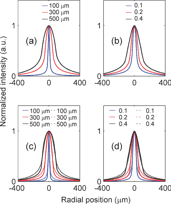 Fig. 7Spatial resolution versus focal plane depth of the (a) absorption and (b) fluorescence imaging for NA of 0.1 (circle), 0.2 (star), and 0.4 (triange), respectively. In (b), straight and dashed lines represent the profiles corresponding to uniform and non-uniform distributions of the fluorescent targets, respectively.  The uniform [straight line, Figs. 6c and 6d] and nonuniform [dashed line, Figs. 6c and 6d] distributions of the fluorescent targets have similar profiles, with the exception that the profile of the nonuniform distribution has slightly longer tails than that of the uniform distribution under the same optical configuration. As discussed below, only fluorescent targets within the top ~500 μm of the tissue have a major effect on the spatial profile. Figures 2c and 2d illustrate that, within the top 500 μm, more fluorescent targets lie in the deeper layers in the nonuniform distribution, resulting in more light scattering and thus longer tails in this case. The spatial profiles of the absorption imaging have longer tails than their fluorescence imaging counterparts under the same optical configuration. Equation 5 indicates that radiance [TeX:] $I_0 (z,\hat \Omega)$ from the incidence light arriving at the point absorber at (0, 0, z) and flowing in the direction [TeX:] $\hat \Omega$ . The point absorber absorbs it and subsequently acts as a negative light source with an emission that propagates toward the detector in the same direction [TeX:] $\hat \Omega$ [Fig. 5a]. Equation 14 describes a similar process for fluorescence imaging except that after the radiance [TeX:] $I_0 (z,\hat \Omega)$ is absorbed, the fluorescent target emits isotropic fluorescence [Fig. 5b]. Because we are interested in light propagating from near to within a few scattering lengths from the surface and the scattering is highly forward (anisotropic factor g is 0.9), the point absorbers act as anisotropic sources that emit radiation preferentially toward deeper tissue layers. Consequently, this light would travel deeper into the tissue and thus experience more scattering as compared to the emission from fluorescent targets that act as isotropic light sources. Therefore, the spatial profile in the former case has longer tails. Figure 7 shows the spatial resolution of absorption (a) and fluorescence imaging (b) versus focal plane depth under different NAs. In both cases, the spatial resolution worsens with the increase of the NA and focal plane depth. Note that the spatial resolutions of absorption and fluorescence imaging are similar, with the exception that those of absorption imaging are slightly worse under the same optical configurations, which is consistent with their spatial profiles. In general, as we vary the NA from 0.1 to 0.4 and the focal plane depth from 20 to 300 μm, we change the spatial resolution from <20 to 200 μm, which is still sufficient to resolve many individual functional columns. For example, the horizontal size of many vertebrate columns ranges from 50 to 800 μm.25 We can compare our result to the spatial resolution obtained by Polimeni using the following tissue parameters: μs0= 35.4 and 53.2 mm−1, μa0= 0.27 and 0.22 mm–1, n0 = 1.4, and g 0 = 0.94 and 0.82 for gray and white matter, respectively; and NA ~0.4 and focal plane depth = 300 μm.9 They used two lenses coupled directly instead of the 4f configuration. They obtained a spatial resolution of 240 μm for the summed contributions within a tissue depth of 200–500 μm.9 This is similar to the 200 μm, which we obtained for NA = 0.4, focal plane depth = 300 μm, and a tissue depth of 200–500 μm. The difference can be attributed to the slight variation in the tissue parameters and the difference between their lenses being directly coupled versus our 4f configuration. The profiles shown in Fig. 6 have larger tails than that of a Gaussian with the same FWHM, which is consistent with that reported by Polimeni.9 Furthermore, Figs. 6c, 6d, 7b show that modifying the density distribution of the fluorescent dyes across the cortical depth from Figs. 2c to 2d can result in a spatial profile with longer tails and yet a slightly smaller FWHM width (i.e., the spatial resolution). This suggests that, in addition to spatial resolution, it is also important to consider a cross talk between signals generated in adjacent cortical columns, which is larger in a case of diffusely reflected light than in the case of Gaussian-like signal profiles. 3.2.Depth Sensitivity Depends on NA and Focal Plane Depth when the Functionally Activated Column is Small and Independent of NA and Focal Plane Depth when the Activated Column is LargeHere, we examine how the NA and focal plane depth affect the depth sensitivity for absorption (Figs. 8 and 9) and fluorescence imaging (Figs. 10 and 11). Figure 8 depicts the depth sensitivity for functionally activated columns of four different cross-sectional areas [Fig. 8a: 10 × 10, Fig. 8b: 50 × 50, Fig. 8c: 100 × 100, and Fig. 8d: 200 × 200 μm2]. In Figs. 8a, 8b, 8c, 8d, NA is fixed at 0.2 and focal plane depth varies among 100 (circle), 300 (star), and 500 μm (triangle). Here, we plot the percent contribution of each layer to the total signal at the detector center using Eqs. 8, 9. For example, for absorption imaging with NA of 0.2 and focal plane depth of 100 μm, the top 100 μm (0–100 μm) of the tissue contributes to ~85% of the total signal (contributions from 0–1000 μm). In Fig. 8a, where the activated column represents a single array of point absorbers [see Fig. 2a] (in our simulation, the horizontal size of one voxel is 10 μm), the depth sensitivity varies drastically with the focal plane depth. In particular, the increase of the focal plane depth from 100 to 300 μm results in a significant increase in the percent contribution from the deeper tissues; the increase of the focal plane depth from 300 to 500 μm, however, results in a smaller increase of the percent contribution from the deeper tissues. For example, the contributions of the tissue within the top 100 μm are 84, 46, and 37%, while those from 200 to 300 μm are 2, 10, and 16%, corresponding to focal plane depths of 100, 300, and 500 μm, respectively. This trend of increasing percent contribution from deeper layers with the focal plane depth reaches a plateau for focal plane depth of >500 μm (not plotted here). Fig. 8Depth sensitivity for functionally activated columns of four different cross-sectional areas: (a) 10 × 10, (b) 50 × 50, (c) 100 × 100, and (d) 200 × 200 μm2, respectively, for absorption imaging. In (a)–(d) NA is fixed at 0.2 and the focal plane depth is varied among 100 (blue), 300 (circle), and 500 (triangle) μm.  Fig. 9Depth sensitivity for functionally activated columns of four different cross-sectional areas: (a) 10 × 10, (b) 50 × 50, (c) 100 × 100, and (d) 200 × 200 μm2, respectively, for absorption imaging. In (a)–(d), the focal plane depth NA is fixed at 300 μm and NA is varied among 0.1 (circle), 0.2 (star), and 0.4 (triangle). 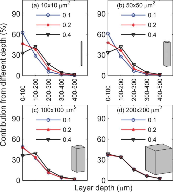 Fig. 10Depth sensitivity for functionally activated columns of four different cross-sectional areas: (a) 10 × 10, (b) 50 × 50, (c) 100 × 100, and (d) 200 × 200 μm2, respectively, for fluorescence imaging with the nonuniform distribution of the fluorescent targets. In (a)–(d), NA is fixed at 0.2 and the focal plane depth is varied among 100 (circle), 300 (star), and 500 (triangle) μm.  Fig. 11Depth sensitivity for functionally activated columns of four different cross-sectional areas: (a) 10 × 10, (b) 50 × 50, (c) 100 × 100, and (d) 200 × 200 μm2, respectively, for fluorescence imaging with the nonuniform distribution of the fluorescent targets. In (a)–(d), the focal plane depth is fixed at 300 μm and NA is varied among 0.1 (circle), 0.2 (star), and 0.4 (triangle). 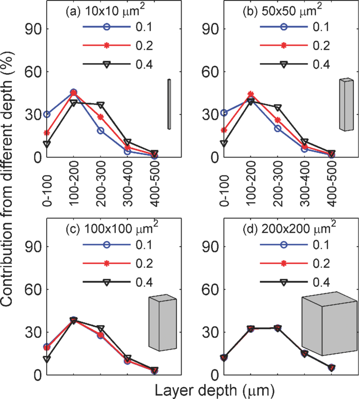 As the cross-sectional area of the activated column increases, the depth sensitivity still varies, but less drastically, with the focal plane depth [Figs. 8b and 8c]. When the area of the activated column reaches 200 × 200 μm2 [Fig. 8d], the depth sensitivity barely depends on the focal plane depth. Note that the horizontal size 200 μm is larger than the spatial resolutions for the given NA and focal plane depths. As can be seen from all panels, >97% of the signal comes from the top 500 μm of tissue; thus, only the depth sensitivity from the top 500 μm is plotted in all panels and the Figs. 8, 9, 10, 11. Figure 9 depicts the depth sensitivity for functionally activated columns with different cross sectional areas [Fig. 9a: 10 × 10, Fig. 9b: 50 × 50, Fig. 9c: 100 × 100, and Fig. 9d: 200 × 200 μm2), when the focal plane depth is fixed at 300 μm and the NA varies between 0.1 (circle), 0.2 (star), and 0.4 (triangle). The results are similar to those of Fig. 8. In Fig. 9a, where the activated column represents a single array of point absorbers, the depth sensitivity varies significantly with the NA. In particular, the increase of the NA from 0.1 to 0.2 results in a large increase of the percent contribution from the deeper tissues; the increase of the NA from 0.2 to 0.4, however, results in a smaller increase of the percent contribution from the deeper tissues. This trend of increasing percent contribution from deeper layers with the NA reaches a plateau for NA ≥ 0.4 (not plotted here). The depth sensitivity for the column with a cross-sectional area of 50 × 50 μm2 [Fig. 9b] is similar to that of [Fig. 9a]. When the area of the activated column increases to 100 × 100 μm2, the depth sensitivity still varies, but less drastically, with the NA. When the area of the activated column reaches 200 × 200 μm2 [Fig. 9d], the depth sensitivity barely depends on the NA. In summary, Figs. 8 and 9 demonstrate that the smaller the cross-sectional area of the activated column is, the more sensitive the depth sensitivity is to the NA and focal plane depth. Interestingly, the depth sensitivity does not depend on the NA or focal plane depth when the horizontal size of an activated column is larger than its spatial resolution, which can be explained as follows: δI z 0(0, 0, z d), the individual contribution to the intensity at the detector center, is proportional to the summation of the Green function G(x, y, z|0, 0, z d) over the cross-sectional area of the activated column. Because this Green function represents the light distribution inside the tissue from a point source at the center of the detector, its summation over a cross-sectional area with a horizontal size larger than spatial resolution is approximately the total power transmitted through the tissue, whose profile versus depth (that is, the depth sensitivity) does not change with either NA or focal plane depth. Next, we present the results for fluorescence imaging. For fluorescence imaging with the uniform distribution of fluorescent targets, these are similar to the results shown in Figs. 8 and 9. Therefore, we only show the results for the nonuniform distribution of fluorescent targets [as depicted in Fig. 2d]. Here, we observe the same trend of the depth sensitivity change with the change of focal plane depth (Fig. 10) and NA (Fig. 11). In addition, there is a notable difference between fluorescence imaging of tissues with uniform and nonuniform staining profile. Figure 10d depicts a higher percent contribution (53%) to the signal from deeper tissues (200–500 μm) than that shown in Fig. 8d (26%), a direct consequence of the different spatial distributions of the fluorescent targets in these two cases, as shown in Figs. 2c and 2d. This illustrates the strong effect of the dye-concentration profile on the depth sensitivity. In many functional fluorescence imaging experiments, the dyes are externally administered. Hence, different dye concentration profiles may be obtained depending on the specific experimental protocols.20, 21, 22 3.3.Larger NA and Focal Plane Depth Suppress the Contribution from Surface Vessels in the Absorption ImagingAs we have seen from Figs. 8d and 10d, the depth sensitivity does not depend on the NA and focal plane depth when the activated column is large. This is only true, however, when the activated columns are devoid of surface vessels above them. In this case, we can assume a uniform distribution of absorption coefficient in the tissue. However, there are areas in the brain tissue that are covered with surface vessels, which can significantly affect the absorption coefficient of that area. Here, we consider only the situation in which the horizontal size of the activated column is larger than the spatial resolution: in particular, in which it is 400 μm. The vessel of 50 × 50 × 50 μm3 is embedded within the top 400 μm of the tissue, and a blood tissue volume ratio of ~1% is used. Hence, the extra point absorbers due to the presence of the vessel is Eq. 19[TeX:] \documentclass[12pt]{minimal}\begin{document}\begin{equation} \delta \mu _{\rm a} (r) = \sum\limits_{\scriptstyle - 25 \le x_i \le 25\,\,{\rm \mu m} \hfill \atop {\scriptstyle - 25 \le y_j \le 25\,\,{\rm \mu m} \hfill \atop \scriptstyle 0 \le z_k \le 50\,\,{\rm \mu m} \hfill}} {100\Delta } \mu _{{\rm a}0} \delta (x - x_i, y - y_j, z - z_k). \end{equation}\end{document}Figure 12a depicts the percent contribution from different depths of tissue and the surface vessel in the absorption imaging for NA of 0.2 and focal plane depths of 100 (circle), 300 (star), and 500 μm (triangle). As we focus deeper into the tissue, the contribution of the surface vessels decreases. For example, the contribution from the surface vessel is suppressed from ~36 to 14% as the focal plane depth changes from 100 to 500 μm. A similar trend is observed for focal plane depth = 300 μm and NA of 0.1 (circle), 0.2 (star), and 0.4 (triangle), as shown in Fig. 12b. Note that when the surface vessels are either very large (≥100 μm) or small (~10 μm), the contribution of the surface vessels to the signal will be either too large or too small; thus, the effect of changing NA and focal plane depth will be negligible. Fig. 12Percent contributions from different depths of the tissue and the surface vessel in the absorption imaging. (a) NA = 0.2 and focal plane depths of 100 (circle), 300 (star), and 500 (triangle) μm. (b) focal plane depth = 300 μm, NA = 0.1 (circle), 0.2 (star), and 0.4 (triangle). In (a, b), the horizontal size of the activated column is 400 μm. The vessel of 50 × 50 × 50 μm3 is embedded within the top tissue and a blood tissue volume of ~1% is used. SV: surface vessel.  Here, we consider absorption imaging only because in many fluorescence imaging experiments the wavelength is chosen so that the absorption of the hemoglobin, and thus, of the surface vessels, is negligible. 4.Discussion4.1.Method validationThe Monte Carlo code tMCimg itself has been validated against an accepted analytic solution for a semi-infinite medium, and cross-validated for a slab geometry with an absorbing inclusion.19 We evoke the first Born approximation in our calculation. In order for this approximation to be valid, the spatial perturbation to the absorption coefficient, δμa(r), needs to be much smaller than the background absorption coefficient μa0.16 As discussed above, δμa(r) is often one order of magnitude smaller than μa(r); thus, the first Born approximation is valid and δI in Eq. 1 can truly represent the difference image. When the perturbation is large, however, a full Monte Carlo simulation needs to be employed. In order to reduce the number of Monte Carlo simulations for calculating the spatial resolution, we take advantage of the 4f configuration so as to simplify Eqs. 5, 10 into Eqs. 6, 14. Here, we examine what will happen if the imaging system does not have a 4f configuration. In general, the two lenses L1 and L2 can have different focal lengths f 1 and f 2, respectively and are separated by a distance d. Let us examine two situations: (i) d = f 1 + f 2 and 2) d ≠ f 1 + f 2. When d = f 1 + f 2, the imaging system can be viewed as a general 4f configuration with magnification M = f 2/f 1. The spatial profiles and spatial resolutions shown in Figs. 6 and 7 are valid as long as we understand that they apply directly to the brain tissue. For example, if M = 2, then a spatial resolution of 200 μm means that we can resolve two cortical columns separated by 200 μm, though on the detector plane they will actually be separated by 400 μm (200 μm × 2). When d ≠ f 1 + f 2, the spatial resolution provides good approximation. For example, the spatial resolution calculated by Polimeni 9 using a tissue model that is similar to a particular configuration used in our simulation, though with a notable difference: in their model, f 1 = f 2, but d ≪ f 1 + f 2, which represents a case very different from the 4f configuration. However, their result of 240 μm is similar to our result of 200 μm. In addition, Orbach and Cohen10 reported an experimental result of 280 μm using a condition similar to that of Polimeni.9 Hence, our simulation improves the efficiency while maintaining results that agree with other calculations and experimental measurements. Note that we do not need to assume a 4f configuration in deriving the equations for calculating depth sensitivity; thus, the depth sensitivity for other optical configurations will be the same as shown in Figs. 8, 9, 10, 11, 12. 4.2.Computational EfficiencyWe have simulated 21 different optical configurations—three values for NA (0.1–0.4) and seven for focal plane depth (20–600 μm)—covering the typical range encountered in camera-based optical brain-imaging experiments. We have considered the optical disturbance within the top 1 mm of the brain tissue and have chosen a voxel size of 10 μm. Therefore, we must calculate the contributions from 100 locations in order to obtain the spatial resolution. As discussed above, in order to obtain the difference images, we calculate the Green function originating from the center of the detector toward the tissue [TeX:] $G(x,y,z,\hat \Omega |0,0,z_{\rm d})$ instead of that originating from the point absorbers (or fluorescent targets) inside the tissue toward the detector [TeX:] $G(x_{\rm d}, y_{\rm d}, z_{\rm d} |0,0,z,\hat \Omega)$ . Here, we will compare the number of simulations needed for both approaches. In the previous case, we need one simulation for each combination of NA and focal plane depth; however, the contributions from different locations inside the tissue are automatically taken care of by [TeX:] $G(x,y,z,\hat \Omega |0,0,z_{\rm d})$ . Hence, we need a total of 21 simulations for estimating the spatial resolution and depth sensitivity of both the absorption and fluorescence imaging. In the latter case, we need 100 simulations. By using the former approach, we improve the efficiency by five times. 4.3.Strategies to Increase the Penetration Depth of Absorption and Fluorescence ImagingAs discussed in Sec. 3, changing NA and focal plane depth does not affect depth sensitivity when the functionally activated cortical areas are large and devoid of large surface vessels. However, as can be seen in Fig. 12, when imaging cortical areas covered with large surface vessels, focusing deeper into the tissue and/or enlarging the NA may suppress the contributions from these vessels and effectively enhance the penetration depth of the absorption imaging. In fact, this practice has been employed in functional imaging to reduce the effect of the surface vessels, as demonstrated in Ref. 15. In many camera-based optical brain imaging experiments, large cortical areas are often excited during the peak response. For example, electrically stimulating the forepaw of a rat can lead to functional activation of a cortical area well beyond 1 mm2. Hence, changing the NA and focal plane depth does not affect the penetration depth (Fig. 8). On the other hand, with the advent of new technologies, such as optogenetics in which optical methods are used to control genetically targeted neurons within intact neural circuits, it is likely that selective activation of a small cross-sectional area ≤ 100 × 100 μm2 may be soon achieved.26 As shown in Figs. 8, 9, 10, 11, focusing deeper into the tissue and/or enlarging the NA would enhance the penetration depth of both absorption and fluorescence imaging of such small cortical areas. In fluorescence imaging, where dyes are applied externally, it may be possible to enhance the contributions from specific cortical layers by regulating the density distribution of the dyes across the cortical depth. For example, in voltage sensitive dye imaging, Ferezou 20 reported a density distribution shown in Fig. 2d, where deeper layers (200–500 μm) had more dye than the shallow layers (0–200 μm). Therefore, the image would consist of more contribution from deeper layers [comparing the two profiles of the depth sensitivity, in Figs. 8d and 10d].20 4.4.Depth Sensitivity is Important in Data Interpretation, Cross Modality and Species Comparison of Functional Imaging ResultsIt is common to compare functional brain-imaging data from different imaging modalities (such as IOI and VSDI) or across species (such as mouse and rat). In general, the mammalian neo-cortex consists of six layers, each with a unique thickness depending on the species and cortical areas.27 To compare fairly, data collected from different modalities or species should come from the same cortical layer(s). Hence, it is critical to know quantitatively the contribution from each layer with a specific imaging modality (e.g., IOI) on a particular animal model (e.g., mouse). Here, we discuss two examples and determine for each whether it is appropriate to compare data obtained from two different modalities or species. We first compare the data from the primary somato-sensory cortex (SI) of a rat obtained from two different modalities: IOI and VSDI. For simplicity, we only consider the case when the activated column is larger than or equal to the spatial resolution and the staining profile for VSDI is nonuniform, as shown in Fig. 2d. As discussed earlier, 97% of the contribution to the signal comes from the top 500 μm. Therefore, we need to consider only layer I (0–150 μm) and II/III (150–650 μm) of the rat SI.27 By using Eqs. 8, 9 for IOI and Eqs. 17, 18 for VSDI, we have obtained the percent contribution from layer I and II/III to the total signal to be 58 and 41% when using IOI, and 26 and 73% when using VSDI. Hence, although the signal is dominated by layer I in IOI, it is dominated by layer II/III in VSDI. The second example examines the IOI results obtained from the same area of two different species: the SI of a mouse and a rat. For simplicity, we only consider the case when the activated column is larger than the spatial resolution. The quantitative analysis of the depth sensitivity shows that 38 and 56% of the signal are from layer I (0–100 μm) and II/III (100–400 μm) of the mouse SI, respectively.27 Once again, although we see that the signal is dominated by layer I in the rat, it is dominated by layer II/III in the mouse. Both examples reveal that caution has to be taken in comparing data across modalities and species. In general, we need to estimate the contribution from each cortical layer of an individual case in order to compare meaningfully data across different imaging modality and species. 4.5.Knowledge of Spatial Resolution and Depth Sensitivity Helps Guide Optical Imaging OptimizationWhen choosing a camera-based optical imaging system, we need to consider important parameters such as NA, focal plane depth, and pixel size of the detector. Our results (Figs. 7, 8, 9, 10, 11, 12) provide both qualitative and quantitative guidance as to how to optimize these parameters: the increase of NA and focal plane depth results in a lower spatial resolution, more suppression of the contribution from the surface vessels, and more contribution from deeper tissues (when the activated column is sufficiently small). In general, larger NA also leads to a stronger signal. Here, we consider some typical examples and give quantitative estimation for each case, as follows:
5.SummaryWe have estimated the spatial resolution and the depth sensitivity of the camera-based 2-D optical imaging methods for a wide range of optical configurations (NA: 0.1–0.4; focal plane depth: 20–600 μm). We have found the following: (i) the spatial resolution worsens with increases in NA and focal plane depth; (ii) for NA ≤ 0.2 or focal plane depth ≤ 300 μm, the spatial resolution is <200 μm, sufficient to resolve individual functional columns; (iii) for functional imaging applications with large activated columns devoid of surface vessels, increasing NA and focal plane depth does not increase the contribution from deeper tissues, but rather reduces the spatial resolution; (iv) increasing NA and focal plane depth may improve the contribution from deeper tissues when small columns are activated or when activated columns are covered with large surface vessels; and (v) our results offer guidance in data interpretation and cross-species/modality comparison, as well as in the optimization of optical imaging configurations. AcknowledgmentsWe thank Ivan Teng and Dr. Qianqian Fang for their help on the simulation program. We gratefully acknowledge support from the NINDS (Grant Nos. NS-051188 and NS-057198 to A. D. and Grant No. NS-057476 to D. A. B.) and NIBIB (Grant No. EB-009118 to A. MD.). We also acknowledge the support from John Carroll University through the Summer Research Fellowship to P. T. ReferencesA. Villringer and
B. Chance,
“Non-invasive optical spectroscopy and imaging of human brain function,”
Trends. Neurosci., 20
(10), 435
–442
(1997). https://doi.org/10.1016/S0166-2236(97)01132-6 Google Scholar
H. Orig and
A. Villringer,
“Beyond the visible-imaging the human brain with light,”
J. Cerebr. Blood F. Met., 23 1
–18
(2003). https://doi.org/10.1097/00004647-200301000-00001 Google Scholar
A. Grinvald, D. Shoham, A. Shmuel, D. Glaser, I. Vanzetta, E. Shtoyerman, H. Slovin, A. Sterkin, C. Wijnbergen, R. Hildesheim, and
A. Arieli,
“In-vivo Optical imaging of cortical architecture and dynamics,”
Modern Techniques in Neuroscience Research, 893
–969 Springer, New York
(1999). Google Scholar
A. Grinvald and
R. Hildesheim,
“VSDI: A new era in functional imaging of cortical dynamics,”
Nat. Rev. Neurosci., 5
(11), 874
–885
(2004). https://doi.org/10.1038/nrn1536 Google Scholar
A. Zepeda, C. Arias, and
F. Sengpiel,
“Optical imaging of intrinsic signals: recent developments in the methodology and its applications,”
J. Neurosci. Meth., 136 1
–21
(2004). https://doi.org/10.1016/j.jneumeth.2004.02.025 Google Scholar
E. M. C. Hillman,
“Optical brain imaging in vivo: techniques and applications from animal to man,”
J. Biomed. Opt., 12
(5), 051402
(2007). https://doi.org/10.1117/1.2789693 Google Scholar
D. Malonek and
A. Grinvald,
“Interactions between electrical activity and cortical microcirculation revealed by imaging spectroscopy: Implications for functional brain mapping,”
Science, 272
(5261), 551
–554
(1996). https://doi.org/10.1126/science.272.5261.551 Google Scholar
I. Vanzetta, H. Slovin, D. B. Omer, and
A. Grinvald,
“Columnar resolution of blood volume and oximetry functional maps in the behaving monkey: Implications for fMRI,”
Neuron, 42
(5), 843
–854
(2004). https://doi.org/10.1016/j.neuron.2004.04.004 Google Scholar
J. R. Polimeni, D. Granquist-Fraser, R. J. Wood, and
E. L. Schwartz,
“Physical limits to spatial resolution of optical recording: clarifying the spatial structure of cortical hypercolumns,”
P. Natl. Acad. Sci. U.S.A., 102
(11), 4158
–4163
(2005). https://doi.org/10.1073/pnas.0500291102 Google Scholar
H. S. Orbach and
L. B. Cohen,
“Optical monitoring of activity from many areas of the in vitro and in vivo salamander olfactory bulb: a new method for studying functional organization in the vertebrate central nervous system,”
J. Neurosci., 3
(11), 2251
–2262
(1983). Google Scholar
B. C. Wilson and
G. Adam,
“A Monte Carlo model for the absorption and flux distributions of light in tissue,”
Med. Phys., 10
(6), 824
–830
(1983). https://doi.org/10.1118/1.595361 Google Scholar
S. A. Prahl, M. Keijzer, S. L. Jacques, and
A. J. Welch,
“A Monte Carlo model of light propagation in tissue,”
Dosimetry of Laser Radiation in Medicine and Biology, 5 102
–111 SPIEVol. IS1989). Google Scholar
S. T. Flock, M. S. Patterson, B. C. Wilson, and
D. R. Wyman,
“Monte Carlo modeling of light propagation in highly scattering tissue—I: model predictions and comparison with diffusion theory,”
IEEE Trans. Biomed. Eng., 36
(12), 1162
–1168
(1989). https://doi.org/10.1109/TBME.1989.1173624 Google Scholar
L. Wang, S. L. Jacques, and
L. Zheng,
“MCML-Monte Carlo modeling of light transport in multi-layered tissues,”
Comput. Meth. Prog. Bio., 47 131
–146
(1995). https://doi.org/10.1016/0169-2607(95)01640-F Google Scholar
E. H. Ratzlaff and
A. Grinvald,
“A tandem-lens epifluorescence macroscope: hundred-fold brightness advantage for wide-field imaging,”
J. Neurosci. Methods, 36
(2-3), 127
–37
(1991). https://doi.org/10.1016/0165-0270(91)90038-2 Google Scholar
A. Dunn and
D. A. Boas,
“Transport-based image reconstruction in turbid media with small source—detector separations,”
Opt. Lett., 25
(24), 1777
–1779
(2000). https://doi.org/10.1364/OL.25.001777 Google Scholar
P. Gonzalez-Rodriguez, A. D. Kim, and
M. Moscoso,
“Reconstructing a thin absorbing obstacle in a half-space of tissue,”
J. Opt. Soc. Am. A., 24
(11), 3456
–3466
(2007). https://doi.org/10.1364/JOSAA.24.003456 Google Scholar
G. Ma, J. Delorme, P. Gallant, and
D. A. Boas,
“Comparison of simplified Monte Carlo simulation and diffusion approximation for the fluorescence signal from phantoms with typical mouse tissue optical properties,”
Appl. Opt., 46
(10), 1686
–1692
(2007). https://doi.org/10.1364/AO.46.001686 Google Scholar
D. Boas, J. Culver, J. Stott, and
A. Dunn,
“Three dimensional Monte Carlo code for photon migration through complex heterogeneous media including the adult human head,”
Opt. Express, 10 159
–170
(2002). Google Scholar
I. Ferezou, S. Bolea, and
C. C. H. Petersen,
“Visualizing the cortical representation of whisker touch: voltage-sensitive dye imaging in freely moving mice,”
Neuron, 50
(4), 617
–629
(2006). https://doi.org/10.1016/j.neuron.2006.03.043 Google Scholar
D. Kleinfeld and
K. R. Delaney,
“Distributed representation of vibrissa movement in the upper layers of somatosensory cortex revealed with voltage-sensitive dyes,”
J. Comp. Neurol., 375 89
–108
(1996). https://doi.org/10.1002/(SICI)1096-9861(19961104)375:1<89::AID-CNE6>3.0.CO;2-K Google Scholar
M. T. Lippert, K. Takagaki, W. Xu, X. Huang, and
J. Wu,
“Methods for voltage-sensitive dye imaging of rat cortical activity with high signal-to-noise ratio,”
J. Neurophysiol., 98 502
–512
(2007). https://doi.org/10.1152/jn.01169.2006 Google Scholar
J. J. Stott and
D. A. Boas, https://orbit.nmr.mgh.harvard.edu/ wiki/index.cgi?tMCimg/README Google Scholar
W. F. Cheong, S. A. Prahl, and
A. J. Welch,
“A review of the optical-properties of biological tissues,”
IEEE J. Quantum Elect., 26
(12), 2166
–2185
(1990). https://doi.org/10.1109/3.64354 Google Scholar
V. B. Mountcastle,
“The columnar organization of the neocortex,”
Brain, 120 701
–722
(1997). https://doi.org/10.1093/brain/120.4.701 Google Scholar
K. Deisseroth, G. Feng, A. K. Majewska, G. Miesenbock, A. Ting, and
M. J. Schnitzer,
“Next-generation optical technologies for illuminating genetically targeted brain circuits,”
J. Neurosci., 26 10380
–10386
(2006). https://doi.org/10.1523/JNEUROSCI.3863-06.2006 Google Scholar
J. J. Hutsler, D. Lee, and
K. K. Porter,
“Comparative analysis of cortical layering and supragranular layer enlargement in rodent carnivore and primate species,”
Brain Res., 1052 71
–81
(2005). https://doi.org/10.1016/j.brainres.2005.06.015 Google Scholar
|


