Real-time blood flow visualization using the graphics processing unit

Laser speckle imaging (LSI) is a noninvasive technique for studying motion of optical scatterers (i.e., red blood cells) with high spatial and temporal resolution. Fercher and Briers¹ first proposed a technique for the analysis of the time-integrated speckle pattern, which results from the interaction of coherent light and a scattering medium. An attractive feature of LSI is its simplicity; the minimum requirements are a laser source, imaging sensor, and a computer for image acquisition and postprocessing. Recently, LSI has found uses in monitoring blood flow in the brain,² retina,³ and skin.^4- 5

Conversion of raw laser speckle images to speckle contrast (SC) and speckle flow index (SFI) images is computationally intensive and CPU-based algorithms are not well suited for real-time processing of high-resolution images, let alone real-time visualization of the postprocessed images. One of the reasons for the slow processing times is that the architecture of modern CPUs is optimized for execution of sequential code, with only a fraction of CPU transistors dedicated to arithmetic operations. On the other hand, graphical processing units (GPUs) are well suited for executing mathematical computations on large data sets in parallel, such as rendering graphics for display on a monitor. In addition, multiple GPUs can be added to a system and processing power will scale nearly proportionally.

To exploit the parallel processing power of GPUs for general purpose computing on GPUs, we used NVIDIA's Compute Unified Device Architecture (CUDA). CUDA allows users with programming knowledge of high-level languages, such as C, to take control of the many stream processors of a GPU using the supplied CUDA C extensions.⁶ Recently, Liu et al. ⁷ utilized CUDA to process laser speckle images and were able to obtain a significant speed-up in processing times. However, the algorithms implemented to do so were not clearly defined and a comparison to a fast and efficient CPU algorithm was not addressed. Here, we describe the GPU algorithm in detail and compare the results to an efficient CPU algorithm. In addition, we describe integration of our GPU-based solution with LSI hardware to achieve a complete, real-time blood flow imaging instrument. To enable end users to integrate our GPU-based approach, the CUDA C source code (Appendix A), “Roll” Algorithm C source code (Appendix B), and LabVIEW real-time demonstration software are available for download from our laboratory's website: http://choi.bli.uci.edu.

In this section, we describe our LSI instrument, the algorithms used to integrate GPU processing into the setup, and visualization of processed images.

Figure 1 shows the setup for our real-time LSI system. The laser used for our experimental setup was a continuous-wave HeNe laser (λ = 633 nm, 30 nm, 30 mW; Edmund Industrial Optics, Barrington, New Jersey). Laser light was delivered to the target with an optical fiber and diverged with a ground-glass diffuser (Thorlabs, Newton, New Jersey). Reflected speckle patterns were imaged with a 12-bit, thermoelectrically cooled CCD Camera (RetigaEXi or Retiga 2000R, QImaging, Burnaby, BC, Canada) with a resolution of 1392 (W)×1040 (H) (Retiga EXi) or 1600 (W)×1200 (H) (Retiga 2000R) pixels and a close-focus zoom lens (18–108 mm, f/2.5-close, Edmund Optics, model no. 52–274, Barrington, New Jersey). Images were transferred to the personal computer (PC) in real time via the FireWire 400 interface at a frame rate of ∼9.7 fps (RetigaEXi) or 8.3 fps (Retiga 2000R). The PC was running an Intel Core 2 4300 running at 1.80 Ghz, 1 GB DDR2 RAM, and Windows XP Professional with Service Pack 3. To process and render the SC and SFI images, we developed software in Microsoft Visual Studio 2005 and LabVIEW 8.6 (National Instruments, Austin, Texas). The graphics card used for image processing was the GeForce 8800GTS made by EVGA, which included the NVIDIA G80 GPU and 640MB of GDDR3 RAM. The performance specifications included a core clock of 500 MHz, memory clock of 800 MHz, shader clock of 1200 MHz, 12 stream multiprocessors, and 96 stream processors (eight per multiprocessor).

To quantify the blurring effect associated with moving particles in raw laser speckle images, the local spatial SC is computed for each pixel using the sliding-window technique (where ω is the radius of the window, usually ω = 2 or ω = 3) and the following: Display Formula

In brief, to relate SC to actual flow rates, the speckle correlation time τ must first be determined. We employed the simplified speckle imaging equation by Ramirez-San-Juan et al. ⁸ and Cheng and Duong:⁹Display Formula

The motivation for using a GPU for this application is its massively parallel architecture, which can be efficiently exploited to compute SC and SFI values much faster than the CPU alone. A raw speckle image is divided into a grid of blocks, called thread blocks, which are processed concurrently by the stream multiprocessors until all blocks are in use. Each multiprocessor has eight stream processors and limited, but extremely fast, on-chip shared memory to be used in the processing of the data in each thread block. To handle the concurrent execution of same command for each thread, NVIDIA uses a new architecture based on single-instruction, multiple-thread that handles the vast number of thread programs in parallel. For this particular application, each thread in the thread block executes identical instructions (called the kernel) for each pixel. Optics-related applications of GPU technology include holography,^10- 11 real-time shape measurements,¹² atmospheric turbulence,¹³ and Monte Carlo modeling of light transport.^14- 15 An excellent description of GPUs is provided in Ref. ¹⁶.

Figure 2 depicts a comparison of CPU and GPU methods to convert a single raw speckle image (e.g., 1392×1040) into SC and SFI images. After the main (host) memory has been allocated, the first step for processing raw speckle images on the GPU is to allocate global memory on the graphics card using the cudaMalloc() function. The raw speckle image, SC, and SFI images are both preallocated, along with intermediate temporary matrices. The raw speckle image is then transferred from host memory to GPU memory using the cudaMemcpy() that was preallocated in the previous step. Next, a grid of thread blocks and number of threads per block must be defined, using the dim3 class, prior to execution of the kernel. Once these variables are defined, the kernel(s) (explained in detail later) can be executed. The SC and SFI images are then moved from GPU memory to host memory using the cudaMemcpy() function. Finally, GPU memory is deallocated using the cudaFree() function.

The conversion from raw speckle images to SC and SFI images consists of two separate kernels (C source code is shown in Appendix A), which collectively mimic the separable convolution method for filters and computes the sum of squares for the standard deviation calculations in Eq. 1 using the least amount of computational resources. The first kernel commences by moving data from global GPU memory to the allocated shared memory and then calculates the sum of the row within the sliding window in which the pixel of interest resides (Fig. 3 depicts a ω = 2 sliding-window example). The second kernel similarly initializes shared memory then computes the sum of the aforementioned summed rows to compute squared sums and mean intensity of the sliding window, with minimal numerical calculations (Fig. 4). The second kernel continues by computing the sample standard deviation in the numerator of Eq. 1. After the SC has been computed for each pixel, a quick calculation using Eq. 3 results in an SFI map.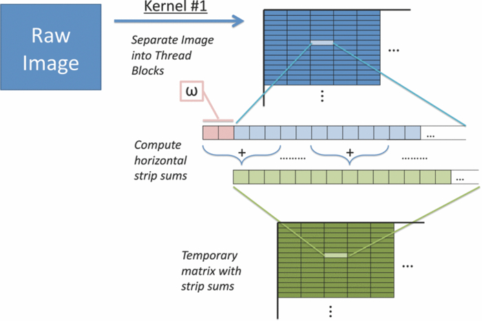

Because of the relative ease of interfacing our QImaging camera with the computer and displaying both raw and processed images, LabVIEW was employed as the visualization platform for our GPU code. To integrate the LSI CUDA C code into LabVIEW, three C wrapper functions are written: LSIonGPU_init(), to initialize the memory on the graphics card, LSIonGPU_process(), to transfer the raw speckle image into GPU space, execute both kernels, and transfer the SC and SFI images back to the host, and lastly LSIonGPU_term() to deallocate GPU memory so that it can be used for other purposes. The entire C project is compiled as a dynamic link library (DLL) so that the functions can be called from LabVIEW.

For maximum performance, LabVIEW code is written with two main while loops, one for image acquisition from the attached camera and another for image processing, which are executed simultaneously (Fig. 5). The purpose for this approach is to enable simultaneous acquisition and processing of images (executed in parallel on a dual-core machine), thus maximizing the frame rate of the system. For this approach to perform properly, a ring buffer must be employed. A ring buffer allocates sufficient memory such that multiple raw images can fit within it. As a new image is acquired, it fills the next space within the buffer and when it reaches the end, it loops around and replaces the first slot, then second, etc. This method aids in ensuring that the processing while loop has enough time to process the data before being replaced by freshly acquired images from the camera.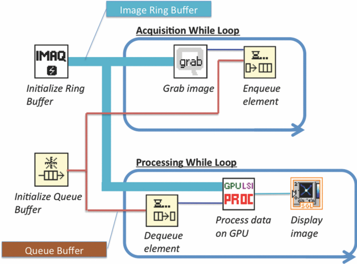

Another important feature in the design of this program is the use of the queue buffer feature in LabVIEW. A queue buffer allows the transfer of data between different parts of a block diagram—in this case, the two while loops. As soon as an image is acquired from the camera and placed into the ring buffer, an element is enqueued into the queue buffer with a reference to the location in which the image was placed. As soon as an element is within the queue buffer, the processing while loop will dequeue the foremost element and can immediately begin processing the dequeued data. These two features in combination allow immediate processing of raw speckle images without the downtime of waiting for processing to finish before a new image is acquired from the camera. As long as the processing time is shorter than the image acquisition time, the proposed algorithm can execute indefinitely.

This section discusses the results of integrating the GPU into the laser speckle image processing model. As a proof of concept, video demonstrations utilizing the custom LabVIEW program are shown.

To make a proper comparison between the performances of a CPU versus a GPU, an efficient CPU algorithm was implemented beforehand. Tom et al. ¹⁷ devised an algorithm named the “Roll” algorithm to convert raw speckle images into SC images. The algorithm takes the rolling sums of rows and columns and subtracts the new row/column to minimize the number of calculations needed to compute the standard deviation of the sliding window. We integrated their algorithm in customized C code and performed benchmarking experiments (C source code is shown in Appendix B).

The timer used to measure system performance for both CPU and GPU algorithms was the built-in timer function in CUDA. Both the CPU and GPU method used a 5×5 sliding-window filter and was performed on randomly generated images generated in C using the rand() function. The results for processing a single image at various image resolutions are displayed in Fig. 6 and compiled in Table 1. For CPU algorithm benchmarking, we exclude the time it takes to allocate free memory due to the fact that the our LabVIEW code only allocates/deallocates memory one time after the program has started, thus making the associated memory management time irrelevant in real-time execution of our code. Similarly, the GPU benchmarking values exclude the time it takes to allocate and deallocate memory on the GPU in addition to the host memory deallocation/allocation times due to the fact that these processes are only performed once during run time. It is important to note that the GPU algorithm times only include the time it takes to transfer the raw image onto the GPU, execute both kernels, and transfer the processed image back to main memory. The normalized errors [(LSI_CPU – LSI_GPU)/(LSI_CPU)] were computed for all pairs of images and found to be negligible, with errors on the order of 10⁻⁷.

With the setup described in Fig. 1, the LabVIEW software is evaluated with a single raw image (1392×1040) being processed with the GPU and visualized with the built-in Intensity Graph. The maximum frame rate is ∼15 fps, which is sufficient to display the real-time LSI images because the maximum frame rate of our camera is ∼10 fps (RetigaEXi). As such, the program can run indefinitely without memory conflicts because the processing and display times are less than the time between collection of successive raw speckle images. In addition, as GPUs gain fast clock speeds, more processing cores, and faster RAM, the gap will widen further.

This section contains videos of the fully functional LabVIEW software described in Section 2c. The videos are acquired with a simple screen capture utility that captures the entire LabVIEW window frame. Videos are taken with ambient lighting off and exposure time set to 10 ms. Please note that the video-capture software in conjunction with a relatively high overhead program, such as LabVIEW, slightly reduces the image-processing speed of the system by ∼1 fps.

The first demonstration consists of viewing real-time SFI images displayed in LabVIEW's built-in Intensity Graph of a reactive hyperemia experiment of the inner hand (¹). A pressure cuff was placed over the upper arm of a subject (IRB Protocol no. 2004‐3626). The palm side of the subject's hand was imaged for 3 min without any applied pressure. The cuff was inflated to 220 mm Hg for 3 min, after which the applied pressure was abruptly released. ¹ shows real-time SFI images collected during the ∼20 s before the pressure cuff was released and the ensuing ∼20 s after release. Immediately after release of the pressure cuff, a typical hyperemic response was observed, with a large-scale influx of blood into the hand.

The second real-time demonstration involves use of the same instrument and software to image, in real-time, ordered fluid flow (²). A simple ordered-flow phantom was created by attaching plastic tubing to a piece of cardboard. The video depicts manually controlled injection of a scattering fluid (20% Intralipid) into the tube with a syringe, followed by manual retraction of the fluid halfway through the video. The position of the leading edge of the fluid moving through the tube can be visualized with high temporal resolution, limited in this case only by the maximum frame rate (∼10 fps) of the camera.

Port wine stain (PWS) birthmarks are vascular malformations characterized by ectatic blood vessels in the dermis of the skin.¹⁸ PWS therapy involves the use of a laser to photocoagulate the blood vessels using a wavelength with high oxy-hemoglobin absorption [e.g., pulsed dye laser (PDL), 577 nm].¹⁹ The LSI system (using the Retiga 2000R camera) was brought into the operating room of the Surgery Laser Clinic adjoining Beckman Laser Institute, and screen-capture video was recorded before, during, and after PDL treatment of PWS. All imaging procedures were approved by the Institutional Review Board at University of California, Irvine (³) depicts the changes in SFI values in the skin of treated areas. The hand of the surgeon and PDL handpiece are intermittently shown within the video footage. The reduction in relative blood flow is immediately apparent and visible for the surgeon to make an assessment of the degree of photocoagulation of PWS vessels.

We have demonstrated a full implementation of real-time visualization of blood flow, using the GPU as the main processing unit and integrated the technology into a LabVIEW-based program. The parallelized architecture of the GPU is able to process data faster than the acquisition rate of our camera and results in our system being limited by the bus speed of the camera. Thus, parallel acquisition and processing of data using the GPU allows for an efficient method for real-time visualization of laser speckle images.

Although the video demos presented here have a slight decrease in visualized frame per second, this is mainly due to the processing overhead associated with LabVIEW. The algorithm to process data is certainly capable of higher frame rates. This system can also be modified with a higher-frame-rate camera while still maintaining very high frame rates. For example, if a 1920 (W)×1440 (H) camera was used, the GPU-based system can process data at ∼30 fps, whereas a CPU-only–based system will result in ∼4 fps. In addition, the flexibility of CUDA enables increased processing speed simply by integrating additional GPUs into the system.

We have also demonstrated the effectiveness of our system by monitoring real-time LSI processed images (³). The relative changes in motion on a macroscopic scale can be visualized for both bulk perfusion and ordered fluid flow. Additionally, preliminary measurements with our real-time LSI system during PWS treatment clearly show a reduction in blood flow, as one would expect with PDL therapy. Therefore, we envision immediate biomedical applications of such an instrument toward image-guided surgery and physiological studies.

// = = = = = = = = = = = = = = = = = = = = = = = = = = = = = = = = = = = =

// Kernel Code that is executed on GPU to convert Raw to SC/SFI

// Two kernels (rows and columns) execute sequentially

// = = = = = = = = = = = = = = = = = = = = = = = = = = = = = = = = = = = =

// 24-bit multiplication is faster on G80,

// but we must be sure to multiply integers

// only within [-8M, 8M - 1] range

#define IMUL(a, b) __mul24(a, b)

#ifndef _SPECKLECONTRAST_H_

#define _SPECKLECONTRAST_H_

////////////////////////////////////////////////////////////////////////////////////////

// Kernel configuration (constants for GPU calculations)

////////////////////////////////////////////////////////////////////////////////////////

// Assuming ROW_TILE_W, KERNEL_RADIUS_ALIGNED and dataW

// are multiples of maximum coalescable read/write size,

// all global memory operations are coalesced in convolutionRowGPU5()

#defineROW_TILE_W 128

#define WINDOW_RADIUS_ALIGNED 16

// Assuming COLUMN_TILE_W and dataW are multiples

// of maximum coalescable read/write size, all global memory operations

// are coalesced in convolutionColumnGPU5()

#define COLUMN_TILE_W 16

#define COLUMN_TILE_H 48

////////////////////////////////////////////////////////////////////////////////////////

// Loop unrolling templates, needed for best performance (5×5 window)

////////////////////////////////////////////////////////////////////////////////////////

template<int i> __device__ int convolutionRowMeans5(int *data){

return data[2 - i] + convolutionRowMeans5<i - 1>(data);

}

template<> __device__ int convolutionRowMeans5<-1>(int *data){

return 0;

}

template<int i> __device__ int convolutionRowSquares5(int *data){

return data[2 - i] * data[2 - i] + convolutionRowSquares5<i - 1>(data);

}

template<> __device__ int convolutionRowSquares5<-1>(int *data){

return 0;

}

template<int i> __device__ int convolutionColumnFull5(int *data){

return data[(2 - i) * COLUMN_TILE_W] + convolutionColumnFull5<i - 1>(data);

}

template<> __device__ int convolutionColumnFull5<-1>(int *data){

return 0;

}

////////////////////////////////////////////////////////////////////////////////////////

// Row convolution filter (5×5)

////////////////////////////////////////////////////////////////////////////////////////

// dataW and dataH are the width and height of raw data, respectively

// d_Data, d_Means, d_Squares are preallocated device memory for the raw input,

//strip sums of mean buffer, and strip sums of squares buffer, respectively

// WINDOW_RADIUS is NOT current implemented, 5×5 window filter is hardcoded

__global__ void convolutionRowGPU5(

int *d_Data,

int *d_Means,

 int *d_Squares,

int dataW,

int dataH,

 int WINDOW_RADIUS

){

// Shared memory allocation

__shared__ int data[2 + ROW_TILE_W + 2];

// Current tile and apron limits, relative to row start

const int  tileStart = IMUL(blockIdx.x, ROW_TILE_W);

const int  tileEnd = tileStart + ROW_TILE_W - 1;

const int  apronStart = tileStart - 2;

const int  apronEnd = tileEnd + 2;

// Clamp tile and apron limits by image borders

const int tileEndClamped = min(tileEnd, dataW - 1);

const int apronStartClamped = max(apronStart, 0);

const int apronEndClamped = min(apronEnd, dataW - 1);

// Row start index in d_Data[]

const int rowStart = IMUL(blockIdx.y, dataW);

// Aligned apron start. Assuming dataW and ROW_TILE_W are multiples

// of half-warp size, rowStart + apronStartAligned is also a

// multiple of half-warp size, thus having proper alignment

// for coalesced d_Data[] read.

const int apronStartAligned = tileStart - WINDOW_RADIUS_ALIGNED;

// Current load postion (of this thread)

const int loadPos = apronStartAligned + threadIdx.x;

// Set the entire data cache contents

// Load global memory values, if indices are within the image borders,

// or initialize with zeroes otherwise

if(loadPos > = apronStart){

 //shared memory postion

 const int smemPos = loadPos - apronStart;

 data[smemPos] =

  ((loadPos > = apronStartClamped) && (loadPos < = apronEndClamped)) ?

  d_Data[rowStart + loadPos] : 0;

 }

// Ensure the completeness of the loading stage

// because results, emitted by each thread depend on the data,

// loaded by another threads

__syncthreads();

// Current write position

const int writePos = tileStart + threadIdx.x;

// Assuming dataW and ROW_TILE_W are multiples of half-warp size,

// rowStart + tileStart is also a multiple of half-warp size,

// thus having proper alignment for coalesced d_Result[] write.

if(writePos < = tileEndClamped){

 const int smemPos = writePos - apronStart;

 int sumMeans = 0;

 int sumSquares = 0;

// Loop unrolling section - computes rolling sums and square sums

// only uses unrolling templates (defined at begining) if defined

// if not defined, uses for loop

#ifdef UNROLL_INNER

 sumMeans = convolutionRowMeans5<2 * 2>(data + smemPos);

 sumSquares = convolutionRowSquares5<2 * 2>(data + smemPos);

#else

 for(int k = -2; k < = 2; k++){

  sumMeans + = data[smemPos + k];

  sumSquares + = data[smemPos + k] * data[smemPos + k];

  }

#endif

   // Writes the strip sums to preallocated global memory

  d_Means[rowStart + writePos] = sumMeans;

   d_Squares[rowStart + writePos] = sumSquares;

 }

}

////////////////////////////////////////////////////////////////////////////////////////

// Column convolution filter + Speckle Contrast + Speckle Flow Index (5×5)

////////////////////////////////////////////////////////////////////////////////////////

// dataW and dataH are the width and height of raw data, respectively

// d_MeansRow, d_SquaresRow are preallocated device memory for strip sums of

// mean and squares values obtained in the previous kernel, respectively

// d_MeansFull, d_SquaresFull are preallocated device memory for full sums of

// mean and squares values buffer, respectively

// d_SC, d_SFI are preallocated device memory for speckle contrast and speckle

// flow index values buffer, respectively

// expT is the exposure time of the raw images

// smemStride, gmemStride are the incremental position movement of the

// shared and globably memory processing positions, respectively

// WINDOW_RADIUS is NOT current implemented, 5×5 window filter is hardcoded

__global__ void convolutionColumnGPU5(

int *d_MeansRow,

int *d_SquaresRow,

int *d_MeansFull,

int *d_SquaresFull,

float *d_SC,

float *d_SFI,

int dataW,

int dataH,

int WINDOW_RADIUS,

float expT,

int smemStride,

int gmemStride

){

// Shared memory allocation

__shared__ int rowMeans[COLUMN_TILE_W * (2 + COLUMN_TILE_H + 2)];

__shared__ int rowSquares[COLUMN_TILE_W * (2 + COLUMN_TILE_H + 2)];

// Current tile and apron limits, in rows

const int tileStart = IMUL(blockIdx.y, COLUMN_TILE_H);

const int tileEnd = tileStart + COLUMN_TILE_H - 1;

const int apronStart = tileStart - 2;

const int apronEnd = tileEnd + 2;

// Clamp tile and apron limits by image borders

const int tileEndClamped = min(tileEnd, dataH - 1);

const int apronStartClamped = max(apronStart, 0);

const int apronEndClamped = min(apronEnd, dataH - 1);

// Current column index

const int columnStart = IMUL(blockIdx.x, COLUMN_TILE_W) + threadIdx.x;

const int num_WINDOW_ELEMENTS = IMUL(WINDOW_RADIUS+1+WINDOW_RADIUS,

WINDOW_RADIUS+1+WINDOW_RADIUS);

// Shared and global memory indices for current column

int smemPos = IMUL(threadIdx.y, COLUMN_TILE_W) + threadIdx.x;

int gmemPos = IMUL(apronStart + threadIdx.y, dataW) + columnStart;

// Cycle through the entire data cache

// Load global memory values, if indices are within the image borders,

// or initialize with zero otherwise

for(int y = apronStart + threadIdx.y; y < = apronEnd; y + = blockDim.y){

 rowMeans[smemPos] =

 ((y > = apronStartClamped) (y < =  apronEndClamped)) ?

 d_MeansRow[gmemPos] : 0;

 rowSquares[smemPos] =

 ((y > = apronStartClamped) (y < =  apronEndClamped)) ?

 d_SquaresRow[gmemPos] : 0;

 smemPos + = smemStride;

 gmemPos + = gmemStride;

}

// Ensure the completeness of the loading stage

// because results, emitted by each thread depend on the data,

// loaded by another threads

__syncthreads();

// Shared and global memory indices for current column

smemPos = IMUL(threadIdx.y + WINDOW_RADIUS, COLUMN_TILE_W) + threadIdx.x;

gmemPos = IMUL(tileStart + threadIdx.y, dataW) + columnStart;

// Cycle through the tile body, clamped by image borders

// Calculate the sum of the strips sums (and squares)

for(int y = tileStart + threadIdx.y; y < = tileEndClamped; y + = blockDim.y){

 int sumMeansFull = 0;

 int sumSquaresFull = 0;

// Loop unrolling section

// only uses unrolling templates (defined at beginning) if defined

// if not defined, uses for loop

#ifdef UNROLL_INNER

 sumMeansFull = convolutionColumnFull5<2 *  2>(rowMeans + smemPos);

 sumSquaresFull = convolutionColumnFull5<2 * 2>  (rowSquares + smemPos);

#else

for(int k = -2; k < = 2; k++){

 sumMeansFull + =

 rowMeans[smemPos + IMUL(k, COLUMN_TILE_W)];

 sumSquaresFull + =

 rowSquares[smemPos + IMUL(k, COLUMN_ TILE_W)];

}

#endif

 // Write sums to device memory

 d_MeansFull[gmemPos] = sumMeansFull;

 d_SquaresFull[gmemPos] = sumSquaresFull;

 // Calcuation of Speckle Contrast (K)

 // K = standard deviation / mean

 // Compute mean

 float mean = sumMeansFull/(float)num_WINDOW_ELEMENTS;