|
|
1.IntroductionExogenous fluorescent probes are increasingly being considered as an alternative to endogenous autofluorescence (AF) contrast for real-time molecular imaging in vivo.1, 2 This is particularly promising for the endoscopic detection and differentiation of precancers in mucosal tissues such as in hollow organs.3, 4 In principle, diagnostic information equivalent to biopsies and histopathologic analysis could be obtained in real time with simultaneous imaging of multiple cancer biomarkers targeted by fluorescent probes of different spectral signatures.5 However, multiplexed imaging is difficult with conventional fluorophores due to their small Stokes shifts.6 Unlike most fluorophores, quantum dots (QDs) are very bright, have broad absorption spectra, relatively narrow emission spectra with large Stokes shift, and have, therefore, been proposed as an alternative for multiplexed fluorescence imaging.7 Although advantageous in some respects, the broad absorption spectrum of QDs introduces a new optimization challenge, namely that the illumination wavelength needs to be carefully chosen in order to maximize the image quality.8 For example, Invitrogen (Carlsbad, CA) recommends using a broadband, short-pass excitation filter for in vitro cell imaging with their QDot products. However, for tissue imaging, the effective excitation spectrum of the QDs is strongly modulated by the tissue optical absorption and scattering.9 To quantify these effects, Lim 9 used a semi-analytical mathematical model tailored for the infrared range, where the tissue AF is negligible. Unfortunately, that approach is not fully applicable to the visible range, since the tissue autofluorescence becomes a limiting factor and the photon diffusion approximation may not be adequate. In this regime, to optimize image contrast, one must carefully select the excitation wavelength to maximize the QD signal while minimizing the AF background.8 This is further complicated by the fact that the AF background is also modulated by the tissue optical properties.10 Optical tissue phantoms are valuable tools to tackle such complex optimization problems. However, as highlighted by Pogue,11 perfect phantoms do not exist and their various properties must be prioritized for the specific application. For the excitation wavelength optimization objective, the top priorities are to have tissue-like absorption, scattering and autofluorescence throughout the visible spectrum and precise (<100 μm accuracy) depth control of a subsurface fluorescent target. Precise placement of inclusions within phantoms is no trivial task. One approach is to place solid inclusions in a gelatin matrix, as described by De Grand,12 but the depth precision is not sufficient for our purposes. De Bruin 13 proposed a precise and flexible way of fabricating phantoms using thin (50 μm) solid building blocks that can be arranged to simulate the geometry of interest. Unfortunately, these were not designed to exhibit tissue-like fluorescence. One approach to get broadband, tissue-like properties is to use actual biological materials for the fabrication. For example, Sokolov 14 used a collagen matrix to simulate cervical epithelium and Kennedy 15 used a fibrin matrix enabling the incorporation of biological agents relevant to OCT applications. Similarly, we initially tried to use thin ex vivo tissue sections layered over a buried fluorophore but this approach suffered from significant dehydration-related artifacts.16 Hence, we developed an approach based on mechanically homogenized tissue samples to obtain an aqueous tissue suspension that can be poured into a custom-made tank designed to hold a fluorophore-loaded capillary as the target. This allows precise control of the depth of the fluorophore target by adjusting the volume of overlying homogenate. In practice, we have found it essential to dilute the tissues (with water), to achieve the required depth control. This also reduces the effects of dehydration and coagulation. Dilution allows accurate “scaling” of the optical thickness of the tissue, and so enables subsurface imaging to be more readily simulated. However, dilution also alters the optical properties and the AF signal, so that a significant focus of the present study is to quantify these effects as a function of the homogenate concentration. We thus present Monte Carlo computer simulations that predict the behavior of the fluorescence contrast as a function of dilution and target depth. To our knowledge, this is the first report of a fully quantitative combined experimental and numerical modeling approach examining optimization of subsurface contrast for wide-field, visible fluorescence imaging. This proof-of-principle report represents the first in a series of papers that will extend the present work to detailed studies for a variety of QDs and fluorophores across a wide spectral range and different tissue types, and then to in vivo studies using animal models. A limited preliminary version of this work was recently presented,17 but here it is extended to a more accurate and robust computational model, validated against a series of experiments using diluted liquid phantoms of known fluorescence and optical properties. We first show that the numerical model accurately predicts (1) the behavior of the autofluorescence measured at the phantom surface as a function of concentration, excitation wavelength and imaging geometry and (2) the behavior of the target-to-background ratio (TBR) as a function of phantom dilution and capillary depth. Finally, we present proof-of-principle results in a model tissue (liver) to show how the proposed approach can be used to optimize the contrast given by 600 nm emitting QDs. 2.Methods2.1.Experimental SetupThe experimental system comprised fluorophore-loaded capillaries submerged in homogenized tissue samples, with the fluorescence imaged from the surface. Square capillary tubing (100×100μm inner, 300×300 μm outer dimensions) was purchased from Polymicro Technologies (Phoenix, AZ). Small sections (∼6 cm) were cut with a surgical blade, their polyimide coating removed with a butane flame, cleaned with ethanol and loaded with the contrast agent. Both ends of the capillary were then sealed off with grease to prevent evaporation. The capillary was then clamped between the upper and lower parts of a custom-made open tank (Fig. 1) machined out of clear polymer, with 4 cm inner diameter. The two parts can be secured tightly with four plastic screws, each part having a rubber O-ring (Able-O-Rings & Seals Inc., Weston, ON, Canada). Silicone gel was applied on both rings prior to sealing the tank. The homogenized tissue (or liquid phantom) was then added until the capillary was fully submerged. Fig. 1Experimental design: (a) epifluorescence imaging setup, (b) tank designed for the inclusion of a capillary target in liquid phantoms, (c) cross-section view.  To determine the “zero depth” capillary position, excess fluid was carefully removed with a micropipette until the capillary emerged and broke the surface tension. The capillary depth (z c) could then be controlled by adding more homogenate by pipette, and its value was calculated from the volume and tank area. The depth estimate was also corrected for surface tension effects, as further discussed in Sec. 5.1. 2.2.QD PreparationFor this study, we used 600 nm emitting (CdSe)ZnS QDs dispersed in chloroform as the target fluorophore. These were prepared in-house using a well-established organometallic procedure.18 QD excitation and emission fluorescence spectra [Fig. 2a] were acquired using a scanning spectrofluorometer (Fluorolog 3, Horiba Jobin-Yvon, Edison, NJ). The QDs exhibited peak emission at 602 nm with full width at half maximum of 35 nm. 2.3.Phantom and Tissue PreparationWe prepared the liquid phantom by mixing 32 mL of Intralipid-20% (Baxter Corporation, Toronto, Canada), 0.32 g of Naphthol Green B powder (N7257-25g, Sigma Aldrich, St. Louis, MO) and 0.2 mg of AlexaFluor 568 (A-20003, Invitrogen Canada Inc., Burlington, ON, Canada). The last was used to simulate the background tissue AF. Distilled water was then added to obtain a total volume of 320 mL of stock phantom material. Twenty serial dilutions (C = 5%, 10%, 15%, … , 100% v/v, 30 mL each) were then prepared from this stock. Fresh bovine liver was used as the model tissue in these studies. Liver was chosen for its high blood content and AF, representing the most challenging subsurface detection situation. The tissue was diced and homogenized using a commercial blender. Excessive heat can be generated in the motor and blade due to the high viscosity of the undiluted tissue. Hence, the samples were kept below 45°C at all times by using prerefrigerated (but not frozen) tissue and frequently pausing the blending process, in order to minimize thermal denaturation that can alter the optical properties. Twenty serial dilutions (5%, 10%, 15%, … , 100% v/v, 30 mL each) were then prepared using phosphate buffered saline (PBS). Suspensions below 30% were passed through a sieve to remove fragments larger than ∼100 μm. We measured the optical properties and AF before and after sieving and observed that the procedure had a negligible effect (data not shown). All measurements were performed within a few hours of the homogenization, since time delays of >24 h had a measureable impact on the AF and optical properties (data not shown). 2.4.Optical Property MeasurementsThe phantom and tissue optical properties were measured using a diffuse reflectance fiber-optic probe as previously described in detail by Kim 19 Briefly, the probe illuminates the sample with white light, and measures the diffuse reflectance spectra at three source-detector separations of 260, 520, and 780 μm. Although these distances are small, it is still possible to apply a diffusion approximation model, if it is constrained by a priori knowledge of the spectral signature of the main absorbers, to yield accurate estimates (within 10%) of the optical properties, as shown previously by Kim and as we also confirmed here in the liquid phantoms across a relevant range of absorption (μ a) and reduced scattering coefficients ( [TeX:] $\mu' _s$ ). 2.5.Fluorescence ImagingFluorescence imaging was performed using a custom-made multi-spectral imaging system. A Coolsnap K4 cooled CCD camera (Photometrics, Tucson, AZ, USA) was mounted on an epifluorescence stereomicroscope (MZFLIII, Leica Microsystems, Richmond Hill, ON, Canada). An automated filter wheel (AB304-T, Spectral Products, Putnam, CT) was placed in the excitation arm of the microscope and loaded with 11 excitation filters (385/20, 405/20, 420/20, 436/30, 450/20, 465/20, 480/20, 495/30, 510/20, 525/20, 546/25, where the notation refers to the central wavelength/full width at half maximum (Chroma Technology Corp., Bellows Falls, VT). The camera and filter wheel were controlled synchronously by an in-house Labview program (National Instruments Corp., Austin, TX). A 500-nm longpass and a 600/50 nm bandpass filter were combined on the detection side. Each sample was first imaged at all excitation wavelengths to obtain its AF excitation spectrum, which was then used as the background signal for the QD contrast measurements. The volume of background fluid was first adjusted to the zero depth, then incremented sequentially to increase the capillary depth. Spectral image sets were acquired at each depth. Smaller volume increments were used for the higher optical density samples to obtain better depth resolution. 2.6.Image analysisAll images were normalized to the output spectrum of the excitation lamp L(λ ex) and the exposure time T, yielding measured fluorescence units of counts/μJ. The excitation lamp power was measured for each excitation filter L(λ ex) using a calibrated optical power meter (840-C, Newport, Irvine, CA). All images were also corrected for the camera noise N (measured in the dark). The corrected image intensity is given by: Eq. 1[TeX:] \documentclass[12pt]{minimal}\begin{document}\begin{equation} J\left({i,j} \right) = \frac{{I(i,j) - N}}{{L(\lambda _{ex})T}}, \end{equation}\end{document}Contrast measurements were obtained by defining, within each corrected capillary image [TeX:] $J_T \left({i,j} \right)$ , a region of interest (ROI) corresponding to the capillary target (TR), and then extrapolating the expected value of the background fluorescence (BR) from a co-registered AF-only image [TeX:] $J_B \left({i,j} \right)$ (Fig. 3). Fig. 3Image analysis procedure. (a) Target ROI selected (solid box) within the corrected capillary image: the ROI width is typically 25% of the image width, and its center corresponds to the middle of the excitation beam (crosshair). (b) To evaluate the background signal, an image of the background medium without the target object is taken and an equivalent ROI (relative to the crosshair) is selected. (c) The pixels within the x coordinates of the ROI (between the dashed lines) are averaged along the horizontal direction and plotted along the y axis, where y = 0 is the vertical position of the crosshairs in both images. Images were taken using the liquid phantom at C = 20%, [TeX:] $\lambda_{ex}= 385\, {\rm nm}$ , [TeX:] $\lambda_{em} = 600\, {\rm nm}$ , [TeX:] $z_{c}= 320\, {\rm \mu m}$ , Z = 6X.  The target-to-background ratio (TBR), as a measure of the object contrast, is given by: dividing the target signal value ( [TeX:] $S_{\rm TR} $ ) by the background signal value ( [TeX:] $S_{\rm BR} $ ): Eq. 2[TeX:] \documentclass[12pt]{minimal}\begin{document}\begin{equation} {\rm TBR} = {{S_{\rm TR} } \mathord{\left/ {\vphantom {{S_{\rm TR} } {S_{\rm BR} }}} \right. \kern-\nulldelimiterspace} {S_{\rm BR} }},\end{equation}\end{document}3.Modeling3.1.AF versus DilutionWe used Monte Carlo computer simulations of photon transport to predict the effect of the homogenized tissue concentration on the measured fluorescence spectra. Given the homogenized tissue optical properties, the output of the fluorescence Monte Carlo model, [TeX:] $G_{\! MC} (\mu _{a,ex,em,C}, \mu' _{s,ex,em,C})$ , and a fluorescence excitation-emission matrix (EEM) measured at any concentration C 0 ( [TeX:] $F_{ex,em,C_0 } $ ), the expected fluorescence EEM at concentration C is given by: Eq. 3[TeX:] \documentclass[12pt]{minimal}\begin{document}\begin{eqnarray} &&\hspace*{-1.5pc}F_{MC} (\mu _{a,ex,em}, \mu '_{s,ex,em}, C) \nonumber\\ &&= \frac{{F_{ex,em,C_0 } G_{MC} (\mu _{a,ex,em,C}, \mu '_{s,ex,em,C})}}{{G_{MC} (\mu _{a,ex,em,C_0 }, \mu '_{s,ex,em,C_0 })}}\end{eqnarray}\end{document}Fig. 4Illumination geometry for epifluorescence imaging (left) and the excitation profile used in the Monte Carlo model. The values of D FOV were 1.45, 0.8, 0.6, and 0.4 cm at Z = 1.5, 3, 4, 6X.  The acceptance angle, a determining parameter for the Monte Carlo simulations, is given by: Eq. 4[TeX:] \documentclass[12pt]{minimal}\begin{document}\begin{equation} \varphi _{{\rm max}} (Z) = {\rm arctan}\left[ {\left({D_{\rm lens} - D_{\rm FOV} (Z)} \right)/2W} \right]\end{equation}\end{document}Eq. 5[TeX:] \documentclass[12pt]{minimal}\begin{document}\begin{equation} r_i = \sigma [ {{{{\rm erf}^{ - 1} (\chi _1)} / {\sqrt 2 }}} ]^{1/2} \end{equation}\end{document}Eq. 6[TeX:] \documentclass[12pt]{minimal}\begin{document}\begin{equation} {\rm sin}(\varphi _i) = \chi _2\,{\rm sin}(\varphi _{\rm max})/n_{\rm tissue}, \end{equation}\end{document}A separate Monte Carlo model was used to calculate the escape function of the emitted fluorescence photons, [TeX:] $E_{em} (r,z_s)$ . Here, [TeX:] $z_s $ is the depth of a buried point source along the z axis. We used 50 nonuniformly distributed (higher density towards the surface) values for [TeX:] $z_s $ and later interpolated the results to match the grid of the absorption distribution [TeX:] $A_{ex} (r,z)$ . The fluorescence emitted at the origin is given by: Eq. 7[TeX:] \documentclass[12pt]{minimal}\begin{document}\begin{equation} G_{MC} = \int_0^\infty {\int_0^\infty {2\pi r\mu _{a,f} Y_{ex} \left({r,z} \right)E_{em} (r,z)dr'dz'} }, \end{equation}\end{document}As shown in Fig. 5, the excitation fluence exhibits a slow and smooth decay for shallow depth values, and a super-Gaussian shape corresponding to the excitation beam in the radial direction. The escape function exhibits a very steep decay similar to that of a point source in vacuum (1/4πr 2) at short distances both in the z and r directions. All curves go through a transition region and then decay exponentially at a rate [TeX:] $\mu _{\rm eff} = [ {3\mu _a (\mu _a + \mu' _s)} ]^{1/2} $ that is characteristic of the diffusion regime.22 Fig. 5Typical Monte Carlo results for (a) depth-resolved and (b) radial excitation fluence [TeX:] $Y_{ex}$ (r,z) (solid and dotted lines) and escape function [TeX:] $E_{em}$ (r,z) (dashed lines) for the 20% phantom sample at 3X zoom. For this particular sample the optical properties were [TeX:] $\mu_{a} = 4.97$ , 0.57, 1.77 cm−1 and [TeX:] $\mu' _s$ = 7.81, 5.94, 5.42 cm−1 at 385, 546 and 600 nm, respectively.  3.2.QD Signal versus Capillary DepthHere we present mathematical expressions for the behavior of the measured QD signal as a function capillary depth and phantom dilution. Note that the QD luminescence could not be directly measured since the pixel intensities represent contributions from two main sources of fluorescence: (1) the QD luminescence (X QD) and (2) the background AF (F MC). Thus, the expected target region signal is given by: Eq. 8[TeX:] \documentclass[12pt]{minimal}\begin{document}\begin{equation} X_{\rm TR} = U[ {X_{\rm QD} + F_{\rm MC} } ],\end{equation}\end{document}The detected QD signal (X QD) varies with capillary depth (z c) and phantom concentration (C). The depth dependence of the QD signal, shown in Fig. 6a, is obtained by integrating maps of the absorption [TeX:] $A_{ex} (r,z)$ and reemission [TeX:] $E_{em} (r,z_s)$ over the capillary volume: Eq. 9[TeX:] \documentclass[12pt]{minimal}\begin{document}\begin{equation} F_{ex,em} \left({z_c } \right) = \int_{z_c }^{z_c + 2x_c } {\int_0^\infty {\alpha \left(r \right)rA_{ex} \left({r,z} \right)E_{em} \left({r,z} \right)drdz} }, \end{equation}\end{document}Eq. 10[TeX:] \documentclass[12pt]{minimal}\begin{document}\begin{equation} \alpha \left(r \right) = \left\{ {\begin{array}{*{20}c} &\hspace*{-.2pc} {4\arcsin \left({x_c /r} \right), \quad r > x_c }, \\ &\hspace*{-.4pc} {2\pi, \hspace*{4.6pc} r \le x_c } \\ \end{array}} \right.\end{equation}\end{document}The expected QD signal as a function of capillary depth is given by: where X QD0 is the QD signal measured when the capillary is at the surface (z = 0).3.3.QD Signal versus Phantom DilutionThe fluorescence emitted by the capillary target does not depend solely on the intensity of the primary incident beam, since the excitation light backscattered from the medium must also be taken into account. Depending on the optical properties, the excitation fluence at the surface can be up to several times that of the incident beam.23 An accurate expression for the behavior of X QD0 with respect to C is thus required. A good approximation of the excitation fluence at the surface (Y ex,C) can be obtained by dividing the absorption map by the absorption coefficient of the medium20 Eq. 12[TeX:] \documentclass[12pt]{minimal}\begin{document}\begin{equation} Y_{ex,C} = {{A_{ex} ({r = 0,z = 0,C})} / {\mu _{a,ex,C} }}.\end{equation}\end{document}Eq. 13[TeX:] \documentclass[12pt]{minimal}\begin{document}\begin{equation} R_{ex,C} = {{({Y_{ex,C} - Y_{\rm beam} })} / {Y_{\rm beam} }},\end{equation}\end{document}Eq. 14[TeX:] \documentclass[12pt]{minimal}\begin{document}\begin{equation} Y_{\rm beam} = \left. {\frac{{p\left(r \right)dr}}{{2\pi rdr}}} \right|_{r = 0} = \left. {\frac{{4r\exp [ { - ({{r / \sigma }})^4 } ]}}{{2\pi r\sqrt \pi \sigma ^2 }}} \right|_{r = 0} = 0.359\sigma ^{ - 2} .\end{equation}\end{document}Fig. 6Typical Monte Carlo results for (a) the detected target signal versus capillary depth [TeX:] $F_{ex,em}(z_{c})$ and (b) the backscattering ratio calculated for the liquid phantoms [TeX:] $R_{ex,C}$ versus C.  The total expected QD fluorescence at the surface, X QD0, can now be expressed in terms of the background-free QD fluorescence, [TeX:] $X_{\rm QD0} $ , as: Eq. 15[TeX:] \documentclass[12pt]{minimal}\begin{document}\begin{equation} X_{\rm QD0} = X'_{\rm QD0} [ {1 + R_{ex,C} } ],\end{equation}\end{document}Eq. 16[TeX:] \documentclass[12pt]{minimal}\begin{document}\begin{equation} X_{\rm QD} = X'_{\rm QD0} [ {1 + R_{ex,C} } ]F_{ex,em} \left({z_c } \right).\end{equation}\end{document}Eq. 17[TeX:] \documentclass[12pt]{minimal}\begin{document}\begin{equation} X_{\rm TBR} = \frac{{U[ {X_{\rm QD} + F_{\rm MC} } ]}}{{F_{\rm MC} }} = \frac{{X_{\rm TR} }}{{F_{\rm MC} }}.\end{equation}\end{document}4.Results4.1.Optical PropertiesAs expected, the measured optical properties increased linearly with concentration for the liquid phantoms and were in good agreement (maximum difference < 10%) with the expected values of Naphthol Green measured in a nonscattering solution and Intralipid-20% reported by Staveren 24 [Fig. 7a]. However, the scattering properties of the diluted homogenized liver samples did not behave linearly with dilution factor (Fig. 7). Hence, we used linear and 3rd order polynomial fits to the absorption and scattering measurements, respectively, as inputs to the Monte Carlo model. 4.2.Liquid Phantoms: AF versus DilutionWe compared the Monte Carlo results from Eq. 3 with fluorescence image measurements taken in the liquid phantoms at various dilutions for four different zoom factors. The agreement was good for all zoom factors and phantom dilutions [Fig. 8a] and excitation wavelengths [Fig. 8b]. Note that the fluorescence spectra in Fig. 8b are similar in shape to that of the AlexaFluor 568 dye [Fig. 2a], but that there are noticeable spectral shifts: e.g., the fluorescence is approximately 3.5 times higher at 546 than at 385 nm for the AlexaFluor 568 dye, but this ratio increases to 7 for the 5% phantom and 14 for the 100% phantom, due to the wavelength-dependent optical properties of the medium, particularly the absorption. Fig. 2(a) Fluorescence excitation (dashed lines) and emission (solid lines) spectra of QD600 and AlexaFluor 568. (b) Optical properties of the main absorber (Naphthol Green, dashed line) and scatterer (Intralipid 20%, solid line) for the stock (100%) liquid phantom. (c) Measured optical properties of the 25% liver homogenate.  4.3.Liquid Phantoms: Target Signal.versus DilutionSeven concentration values (C = 5, 10, 15, 20, 40, 60, 80%) were selected from the diluted phantoms and fluorescence imaging was performed at 3X and 6X. The target signal, S TR, was obtained as described in Sec. 2.6 and compared with the results of Eq. 8. There is close agreement between the simulations and measurements over the full range of excitation wavelengths, concentrations and zoom factors tested [Fig. 9a]. Moreover, division by the predicted AF spectra yields accurate estimates for the surface target-to-background ratio. Since the capillary signal is relatively flat in the 385–480 nm region but the AF reaches a minimum at 420–436 nm, the TBR peaks at 420–436 nm for all dilution factors [Fig. 9b]. Fig. 9a clearly shows that the measured capillary signal is a combination of the QD and the background fluorescence. At longer wavelengths (>500 nm), the background fluorescence is dominant and is mainly responsible for the increase of signal with phantom concentration. At shorter wavelengths (<460 nm), the increase in signal is mostly attributable to the effect of the backscattering on the QD fluorescence. Note that these trends are not directly related to the actual wavelength but rather to the shapes of the QD and AlexaFluor 568 excitation spectra. Different fluorophores would yield different trends. Fig. 9Measured (symbols) and calculated (dashed lines) (a) surface capillary signal, X TR0 versus [TeX:] $\lambda_{ex}$ and (b) the corresponding TBR versus [TeX:] $\lambda_{ex}$ results obtained at Z = 6X for various phantom concentrations (C = 5, 10, 15, 20, 40, 60, 80%). The black solid line in (a) represents the corrected background-free quantum dot fluorescence, [TeX:] ${\it UX}' _{\rm QD0}$ . Almost identical results were obtained at Z = 3X (data not shown).  4.4.Liquid Phantoms: Target Signal versus DepthFor each of the seven selected phantoms, we imaged the capillary at increasing depth until it became undetectable due to low contrast ( [TeX:] $S_{\rm TR} \cong S_{\rm BR} $ ). Both the capillary signal and contrast measurements were in good agreement with the models over the range of wavelengths, depths, dilution and zoom factors tested. Fig. 10a shows that the target ROI signal is initially a combination of the background and QD fluorescence, but that the QD component decays rapidly with depth until only the background component remains. Fig. 10b shows a clear maximum region (400–450 nm) in the TBR spectra at zero depth. Note that this region corresponds to a dip in all the phantom AF excitation spectra [Fig. 8b]. Also, the TBR spectra rapidly flatten with depth, as the QD component of the signal decays toward zero. Fig. 8Monte Carlo calculations (dashed lines) and experimental measurements (symbols) in the liquid phantoms. (a) AF versus C for various zoom factors (Z = 1.5, 3, 4, 6X) at [TeX:] $\lambda_{ex}= 465\, {\rm nm}$ and [TeX:] $\lambda_{ex}= 600\, {\rm nm}$ . (b) AF versus [TeX:] $\lambda_{ex}$ for various concentrations (C = 5, 10, 25, 50, 75, 100%) at Z = 6X and [TeX:] $\lambda_{ex}= 600\,{\rm nm}$ . The insert shows the low signal region re-scaled for better viewing. The Monte Carlo results were normalized at [TeX:] $C_{0}$ = 40%. 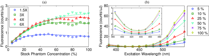 4.5.Homogenized TissuesTo further test the experimental method and modeling, AF and contrast measurements were performed on the diluted homogenized liver samples. The model accurately predicts the shape of the fluorescence versus dilution curves [Fig. 11a] and the slight AF spectral shifts induced by the dilution [Fig. 11b] despite the nonlinear behavior of the scattering coefficient. The models are also in good agreement with the experimental contrast data, for surface and sub-surface capillary measurements [Fig. 11c and 11d]. For surface imaging, peak contrast regions can be observed at 385–420 nm and 510–540 nm. These spectral bands correspond to minima in the liver AF spectra [Fig. 11b]. Another interesting observation is that the TBR spectra flatten rapidly with increasing capillary depth, but at a faster rate in the 385–420 nm region, which results in the 510–540 nm peak surpassing the former at shallow depths. Fig. 11Measured (symbols) and calculated (dashed lines) for (a) liver AF versus C at various [TeX:] $\lambda_{ex}$ , (b) AF versus [TeX:] $\lambda_{ex}$ at various homogenate dilutions, (c) surface TBR versus [TeX:] $\lambda_{ex}$ at C = 25 and 100%, and (d) TBR versus [TeX:] $\lambda_{ex}$ at various capillary depth values for the 25% tissue homogenate. The autofluorescence Monte Carlo results were normalized at [TeX:] $C_{0}$ = 30%.  5.Discussion5.1.ExperimentalThe experimental setup provided a convenient approach to study subsurface fluorescent image contrast in a controlled, tissue-like environment. The liquid optical phantoms allowed accurate control of the absorption, scattering and fluorescence properties of the background medium and an accurate means to vary the depth of the fluorescent target. The setup also allows measurements with diluted tissue homogenates that more truly represent the tissue optical properties and AF spectra. A limitation of the homogenates is the limited shelf-life (<24 h) compared to the artificial phantoms (2–3 weeks) or solid phantoms (months to years13). The capillary structure provides a well delineated fluorescent target for depth-resolved imaging but presents some practical challenges. Given that we are interested in accurate subsurface measurements (<∼500 μm), finding the zero depth position is nontrivial due to surface tension effects. This placed a lower limit of about 200±50 μm on the capillary depths that could be achieved. This problem was observed in two ways. First, at high concentrations (60 and 80%), the initial drop in the QD signal from the surface to the first depth increment was much larger than predicted, but the signal then behaved as expected with further depth increases [Fig. 12b]. Second, in several images, a relatively thick layer of fluid could be seen completely covering the outer segments of the capillary while the center was fully exposed [Fig. 12a], likely due to the surface wetting that starts at the edges of the capillary as the tank is filled. It is worth noting that these surface tension effects were less pronounced for the tissue homogenates. Fig. 12Illustration of the difficulty of determining the exact capillary depth near the phantom surface. (a) Typical fluorescence image showing 60% liquid phantom wetting the capillary on both sides but not covering the center portion. The image was taken at [TeX:] $\lambda_{ex}= 436\, {\rm nm}$ , [TeX:] $\lambda_{ex}= 600\, {\rm nm}$ , Z = 3X, and the expected capillary depth was 80 μm (green squares in b). The calculated (dashed lines) and measured (symbols) data is shown (b) before and (c) after correcting the capillary depth for the surface tension effects.  The 200±50 μm value was empirically derived from the experimental data but the basis for this is not well understood. In theory, the surface energy of fused silica is higher than that of water and perfect wetting should be observed. However, fused silica can be de-activated (reduced surface energy) through various chemical treatments,25 and we may have inadvertently done so during the polyimide coating removal or ethanol cleaning processes. A potential solution would be the use of surfactants to reduce or eliminate the surface tension effects. It would also be useful to include a means of monitoring the capillary depth during the imaging, for example by optical coherence tomography. 5.2.Image and Data AnalysisGiven that the target fluorescent light scatters in the phantom and that the phantom has a 4 cm diameter, we used a separate target-free set of images to determine the background signal and then applied a spatial registration algorithm, rather than using a background ROI at some distance from the capillary. The images were also corrected for the nonuniform excitation light distribution (the intensity can vary 10-fold from the center to the edges), minimizing the correction by limiting the field of view and keeping the target close to the beam center. Straightforward corrections for the spectral output of the lamp and the camera noise were also applied to the images. Once processed, replicate fluorescence measurements were within ±5% for the liquid phantoms and ±15% for the tissue homogenates, the latter variance being due to macroscopic (∼mm) spatial heterogeneities, the occasional presence of air bubbles, and photobleaching of the AF. The uncertainties in the measured absorption and scattering properties were also greater for the tissue homogenates than for the liquid phantoms (<±10%), since the spatially resolved diffuse-reflectance measurement technique19 requires a priori knowledge of the main absorption and scattering spectral shapes. We used both forms of hemoglobin (oxy and de-oxy) as the only absorbers and forced a power-law of the form λ −k with k < 1.5 to fit the scattering spectra.24 While the derived optical properties yielded satisfactory results for the depth and dilution dependence compared to the experiments, there were some discrepancies. For example, in Fig. 11d, the model overestimates the tissue attenuation at 436 nm, which corresponds to a peak in the hemoglobin absorption spectrum. Since the diffuse reflectance is very low when the tissue absorption is high, the signals are near the noise floor of the instrument. The fact that the scattering coefficient of the tissue homogenate increases non-linearly with concentration also needs explanation. This is probably not a measurement artifact, since the behavior is also observed in the AF versus dilution data and confirmed by the Monte Carlo simulations. This could be due to “aggregates” of scattering particles whose size depends on the dilution factor. It is not known if this effect is particular to liver tissue, but it could be tested by light scattering spectroscopy on the diluted tissue samples. 5.3.ModelingSince the Monte Carlo model is in good agreement with the experimental data over a broad range of excitation wavelengths, optical properties, AF background levels and imaging geometries, it could potentially be used, with some degree of confidence, to estimate the behavior of undiluted tissue samples from measurements made on diluted homogenates, as illustrated in Fig. 13. This figure also shows an example of subsurface TBR data calculated at capillary depths that could not be achieved experimentally. Since we do not have subsurface measurements for the 100% liver case, it is difficult to evaluate the accuracy of the modeling results in Fig. 13b, but note that the agreement is within about 20% at the surface, even for this tissue which has very high optical attenuation. Fig. 13Proof-of-principle Monte Carlo evaluation of TBR data to unreachable experimental conditions. (a) for very shallow depths and (b) for nondiluted tissue. 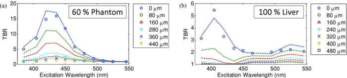 One limitation of the Monte Carlo approach is the computation time required. Most of the simulations presented above were performed using an ANSI C implementation of the MCML code implemented on a CPU cluster (42 nodes × 2 × 3 GHz Intel Xeon processors). A single simulation with 5 million photons required typically 1–30 min, depending on the optical properties, with the highly scattering cases taking longest. However, 20–40 simulations could be run in parallel, so that the total computation time for an entire data set (20 concentrations × 11 excitation wavelengths × 50 source depth values × 1 emission wavelength) was less than 12 h. This could be further reduced by using GPU-acceleration26 or by a hybrid Monte Carlo-diffusion theory approach,27 although the latter may not be useful for subsurface modeling due to violation of diffusion theory boundary conditions. To avoid having to execute a much more complicated Monte Carlo model, the perturbations due to the fluorescent target and the finite capillary wall thickness were not included in the calculation of the excitation or emission fluence distributions. Instead, we used the experimentally derived factor U and obtained satisfactory agreement between the simulated and experimental results throughout the tested parameter space. This was likely due to the small size of the target compared to the phantom and beam dimensions and the low concentration of the QD solutions used (μ a, QD < 1 for all wavelengths), and the effect of the capillary wall thickness did not appear significant. A more complete model would be required for large targets and/or target absorption coefficient much higher than that of the surrounding tissue. For many in vivo applications of interest (fluorescence imaging of microvasculature, dysplasias/early tumors), this is not likely to be the case. 6.ConclusionsWe have shown how phantoms comprising diluted homogenized tissues provide a practical experimental tool to evaluate surface/subsurface imaging of fluorescent contrast agents such as quantum dots. The purpose of diluting the tissue homogenates was to make them easier to handle, particularly for scaling the near-surface depths. While not in itself relevant to subsurface imaging applications, the use of liver (with its high attenuation in the visible range) as a model tissue homogenate demonstrated proof-of-principle of the approach. The Monte Carlo simulations are in good agreement with the experimental results on three levels: the tissue AF with respect to dilution, the target signal as a function of depth, and the target signal as a function of tissue dilution. This gives confidence that the use of phantoms made with dilute tissue homogenates is valid for contrast optimization studies. Moreover, we have observed that the optimal contrast peaks do not spectrally shift significantly with dilution, indicating that valid wavelength-optimization conclusions can be reached without requiring very detailed analysis of the effects of dilution on the tissue optical properties. Finally, the TBR results indicate following conclusions on optimizing the fluorescence image contrast in the surface/subsurface geometry: (1) for surface imaging, maximum contrast is achieved with an excitation wavelength that corresponds to a minimum in the background AF and a maximum in the target excitation spectrum, (2) the background AF spectra are modulated by the tissue optical properties, with absorption peaks usually coinciding with dips in the AF spectrum, (3) for the surface tissue homogenate data the optimal contrast peaks coincide with maxima in the hemoglobin absorption spectrum, (4) the TBR spectra flatten out with target depth at a rate that increases predominantly with tissue absorption, (5) for shallow depth imaging in liver tissue, the TBR exhibits a spectral shift in favor of the 510–540 peak due to the higher tissue absorption at 385–420 nm. We note that some of these conclusions are as would be expected qualitatively a priori. However, the ultimate value of the approach presented here lies in the ability to quantify the effects of factors such as the tissue absorption and scatter on fluorescence contrast measurements. For example, it is generally accepted that using NIR emitting fluorophores yields better image contrast than visible ones due to reduced tissue autofluorescence background,28 but this has not been rigorously quantified, so that the implications for optimizing contrast agent dose are not clear. To address such questions, a follow-up study is in progress that will present detailed and quantitative contrast optimization results obtained from imaging visible and near-infrared QDs and fluorophores in different tissues. A further in vivo study using a dorsal skin fold window chamber mouse model is also underway to determine the critical optimization conditions for fluorescence imaging of micro-vasculature and tumors, with emphasis given to the relationship between the injected dose, measured contrast, and the choice of excitation and emission wavelengths. AcknowledgmentsThis work was supported by the Canadian Institutes of Health Research (CIHR #RMF-72551). M. Roy and A. Kim also received financial support from the Natural Sciences and Engineering Research Council of Canada. Infrastructure support was provided by the Ontario Ministry of Health and Long Term Care: the opinions expressed do not necessarily represent those of OMHLTC. The authors would like to acknowledge Luc Charron, Dr. Paul Constantinou and Dr. Ralph DaCosta for insightful theoretical discussions, Dawei Li and Dr. Wen Jiang and Dr. Warren Chan for providing QDs and QD-related information, Dr. George Netchev and Dr. Robert Weersink for assistance with optical instrumentation, and Sean Davidson and Michael Wood for help with the Monte Carlo simulations. ReferencesM. Ferrari,
“Cancer nanotechnology: opportunities and challenges,”
Nature Rev., 5 161
–171
(2005). https://doi.org/10.1038/nrc1566 Google Scholar
W. Cai, A. Hsu, Z.-B. Li, and
X. Chen,
“Are quantum dots ready for in vivo imaging in human subjects?,”
Nanoscale Res. Lett., 2 265
–281
(2007). https://doi.org/10.1007/s11671-007-9061-9 Google Scholar
R. S. DaCosta, B. C. Wilson, and
N. E. Marcon,
“Optical techniques for the endoscopic detection of dysplastic colonic lesions,”
Curr. Opin. Gastroenterol., 21 70
–79
(2005). Google Scholar
B. C. Wilson,
“Detection and treatment of dysplasia in Barrett's esophagus: a pivotal challenge in translating biophotonics from bench to bedside,”
J. Biomed. Opt., 12 051401
–051422
(2007). https://doi.org/10.1117/1.2795688 Google Scholar
P. L. Hsiung, J. Hardy, S. Friedland, R. Soetikno, C. B. Du, A. P. Wu, P. Sahbaie, J. M. Crawford, A. W. Lowe, C. H. Contag, and
T. D. Wang,
“Detection of colonic dysplasia in vivo using a targeted heptapeptide and confocal microendoscopy,”
Nature Med., 14 454
–458
(2008). https://doi.org/10.1038/nm1692 Google Scholar
I. L. Medintz, H. T. Uyeda, E. R. Goldman, and
H. Mattoussi,
“Quantum dot bioconjugates for imaging, labelling and sensing,”
Nature Mater., 4 435
–446
(2005). https://doi.org/10.1038/nmat1390 Google Scholar
M. Han, X. Gao, J. Z. Su, and
S. Nie,
“Quantum-dot-tagged microbeads for multiplexed optical coding of biomolecules,”
Nat. Biotech., 19 631
–635
(2001). https://doi.org/10.1038/90228 Google Scholar
M. Roy and
B. C. Wilson,
“Molecular imaging with targeted quantum dot bioconjugates: the need for contrast optimisation studies,”
Int. J. Nanotechnol., 6 442
–455
(2009). https://doi.org/10.1504/IJNT.2009.024639 Google Scholar
Y. T. Lim, S. Kim, A. Nakayama, N. E. Stott, M. G. Bawendi, and
J. V. Frangioni,
“Selection of quantum dot wavelengths for biomedical assays and imaging,”
Mol. Imag., 2 50
–64
(2003). https://doi.org/10.1162/153535003765276282 Google Scholar
M. G. Muller, I. Georgakoudi, Q. Zhang, J. Wu, and
M. S. Feld,
“Intrinsic fluorescence spectroscopy in turbid media: disentangling effects of scattering and absorption,”
Appl. Opt., 40 4633
–4646
(2001). https://doi.org/10.1364/AO.40.004633 Google Scholar
B. W. Pogue and
M. S. Patterson,
“Review of tissue simulating phantoms for optical spectroscopy, imaging and dosimetry,”
J. Biomed. Opt., 11 041102
(2006). https://doi.org/10.1117/1.2335429 Google Scholar
A. M. De Grand, S. J. Lomnes, D. S. Lee, M. Pietrzykowski, S. Ohnishi, T. G. Morgan, A. Gogbashian, R. G. Laurence, and
J. V. Frangioni,
“Tissue-like phantoms for near-infrared fluorescence imaging system assessment and the training of surgeons,”
J. Biomed. Opt., 11 014007
(2006). https://doi.org/10.1117/1.2170579 Google Scholar
D. M. de Bruin, R. H. Bremmer, V. M. Kodach, R. de Kinkelder, J. van Marle, T. G. van Leeuwen, and
D. J. Faber,
“Optical phantoms of varying geometry based on thin building blocks with controlled optical properties,”
J. Biomed. Opt., 15 025001
(2010). https://doi.org/10.1117/1.3369003 Google Scholar
K. Sokolov, J. Galvan, A. Myakov, A. Lacy, R. Lotan, and
R. Richards-Kortum,
“Realistic three-dimensional epithelial tissue phantoms for biomedical optics,”
J.Biomed. Opt., 7 148
–156
(2002). https://doi.org/10.1117/1.1427052 Google Scholar
B. F. Kennedy, S. Loitsch, R. A. McLaughlin, L. Scolaro, P. Rigby, and
D. D. Sampson,
“Fibrin phantom for use in optical coherence tomography,”
J. Biomed. Opt., 15 030507
(2010). https://doi.org/10.1117/1.3427249 Google Scholar
M. Roy, R. S. DaCosta, R. Weersink, G. Netchev, S. R. H. Davidson, W. C. W. Chan, and
B. C. Wilson,
“Quantum dots as contrast agents for endoscopy: mathematical modeling and experimental validation of the optimal excitation wavelength,”
Proc. SPIE, 6448 644812
(2007). https://doi.org/10.1117/12.700954 Google Scholar
M. Roy, and
B. C. Wilson,
“An accurate homogenized tissue phantom for broad spectrum autofluorescence studies: a tool for optimizing quantum dot-based contrast agents,”
Proc. SPIE, 6870 68700E
(2008). https://doi.org/10.1117/12.764639 Google Scholar
B. O. Dabbousi, J. Rodriguez-Viejo, F. V. Mikulec, J. R. Heine, H. Mattoussi, R. Ober, K. F. Jensen, and
M. G. Bawendi,
“(CdSe)ZnS Core-Shell Quantum Dots: Synthesis and Characterization of a Size Series of Highly Luminescent Nanocrystallites,”
J. Phys. Chem. B, 101 9463
–9475
(1997). https://doi.org/10.1021/jp971091y Google Scholar
A. Kim, M. Roy, F. Dadani, and
B. C. Wilson,
“A fiberoptic reflectance probe with multiple source-collector separations to increase the dynamic range of derived tissue optical absorption and scattering coefficients,”
Opt. Exp., 18 5580
–5594
(2010). https://doi.org/10.1364/OE.18.005580 Google Scholar
L. Wang, S. L. Jacques, and
L. Zheng,
“MCML–Monte Carlo modeling of light transport in multi-layered tissues,”
Comput. Methods Programs Biomed., 47 131
–146
(1995). https://doi.org/10.1016/0169-2607(95)01640-F Google Scholar
F. P. Bolin, L. E. Preuss, R. C. Taylor, and
R. J. Ference,
“Refractive index of some mammalian tissues using a fiber optic cladding method,”
Appl. Opt., 28 2297
–2303
(1989). https://doi.org/10.1364/AO.28.002297 Google Scholar
T. J. Farrell, M. S. Patterson, and
B. Wilson,
“A diffusion theory model of spatially resolved, steady-state diffuse reflectance for the noninvasive determination of tissue optical properties in vivo,”
Med. Phys., 19 879
–888
(1992). https://doi.org/10.1118/1.596777 Google Scholar
C. M. Gardner, S. L. Jacques, and
A. J. Welch,
“Light transport in tissue: Accurate expressions for one-dimensional fluence rate and escape function based upon Monte Carlo simulation,”
Lasers Surg. Med., 18 129
–138
(1996). https://doi.org/10.1002/(SICI)1096-9101(1996)18:2<129::AID-LSM2>3.0.CO;2-U Google Scholar
H. J. van Staveren, C. J. M. Moes, J. van Marie, S. A. Prahl, and
M. J. C. van Gemert,
“Light scattering in Intralipid-10% in the wavelength range of 400-1100 nm,”
Appl. Opt., 30 4507
–4514
(1991). https://doi.org/10.1364/AO.30.004507 Google Scholar
K. Bartle, B. Wright, and
M. Lee,
“Characterization of glass, quartz, and fused silica capillary column surfaces from contact-angle measurements,”
Chromatographia, 14 387
–397
(1981). https://doi.org/10.1007/BF02262872 Google Scholar
E. Alerstam, T. Svensson, and
S. Andersson-Engels,
“Parallel computing with graphics processing units for high-speed Monte Carlo simulation of photon migration,”
J. Biomed. Opt., 13 060504
–060503
(2008). https://doi.org/10.1117/1.3041496 Google Scholar
B. Luo, and
S. He,
“An improved Monte Carlo diffusion hybrid model for light reflectance by turbid media,”
Opt. Exp., 15 5905
–5918
(2007). https://doi.org/10.1364/OE.15.005905 Google Scholar
X. Gao, L. Yang, J. A. Petros, F. F. Marshall, J. W. Simons, and
S. Nie,
“In vivo molecular and cellular imaging with quantum dots,”
Curr. Opin. Biotechnol., 16 63
–72
(2005). https://doi.org/10.1016/j.copbio.2004.11.003 Google Scholar
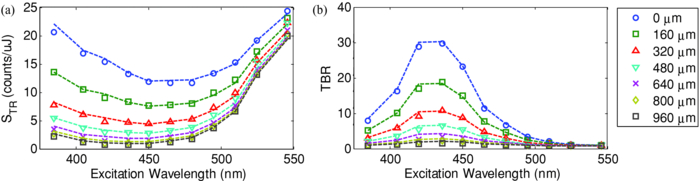
|