1.

Introduction

Coherent anti-Stokes Raman scattering (CARS) is a very powerful method, which has been successfully applied to a vast number of different systems and applications, ranging from small molecules in combustion analysis^{1, 2, 3, 4, 5, 6} to microscopy of complex systems.^{7, 8, 9} Particularly in microscopy, CARS provides labeling free characterization of complex biological systems.^{10, 11} The power of the CARS based microscopy resides on the nonlinear interaction between three laser pulses (pump, Stokes, and probe) which gives rise to a blue-shifted signal (anti-Stokes) with high spatial resolution and potential for chemical selectivity.^{12, 13}

CARS can be implemented in several ways. In a conventional CARS setup, all required frequencies are provided by using two synchronized pulsed lasers with a frequency difference matching to one vibrational level of the sample molecule.¹⁴ Such a demanding setup is simplified by the multiplex CARS (MCARS) approach, where a broadband spectrum covering a whole range of Raman shifts is used instead of a tuneable monochromatic Stokes pulse [Fig. 1a].^{15, 16, 17} Generation of broad supercontinuum has been nicely performed using photonic crystal fibers (PCF),^{18, 19, 20} where unamplified 100 fs-pulses from a standard Ti:Sapphire oscillator can be easily converted into a “white light” spectrum.²¹

Fig. 1

(a) The nonlinear Raman process of MCARS with the interacting electrical fields of the pump-, Stokes-, and probe-beam (ω_p, ω_S, ω_p’, respectively) resulting in the blue shifted anti-Stokes signal (ω_CARS). (b) MCARS experimental setup. BS: Beam splitter, F1: band pass filter cuts out the narrowband pump- and probe-beam, PCF: photonic crystal fiber broadens the Stokes-beam, F2: long pass filter where pump and Stokes are spatially overlaid again, MO1: microscope objective for measurement, MO2: microscope objective for signal output collimation, F3: short pass filter.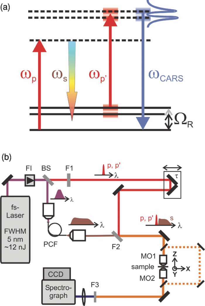

Despite of all the advantages of CARS and the resulting efficient setups now available, there are still issues that have to be addressed for microscopic applications: One of the main experimental challenges is the coherent nature of CARS, which leads to interference between molecular signals and, therefore, to distortion of Raman line intensities and Stokes shifts. In order to obtain similar information as provided by the classical Raman spectroscopy, the imaginary part of the complex third order susceptibility of CARS has to be separately extracted. Although this issue has been addressed by several promising techniques, e.g., by the maximum entropy method,^{22, 23} the implementation of such mathematical analysis is not widespread. This has been a limiting factor particularly in image contrast of biological samples, restricting the analysis to strong single spectral features directly taken from the raw data, like the amplitude of the CH-stretching vibration of lipids at about 2900 cm⁻¹.^{24, 25} Although this single-channel approach is fast and easy to apply, spectral information blue shifted to the strongest signal is often suppressed by the dispersive lineshape, leading potentially to a loss of important spectral information. Moreover, particularly in the case of multiplex broadband data acquisition, which provides spectral information over a range of more than 2500 cm⁻¹,²⁶ it would be desirable to have an imaging procedure that is sensitive to every spectral information that might occur within the detected range. This subject is directly associated to the second challenge of data processing, namely to discriminate between noise and spectral features that belong to different sample components. When the pure chemical components of the sample are known, they can be separately measured in order to fit the complex MCARS spectrum. Thus, it is possible to analyze the hyperspectral data, e.g., using an evolutionary fitting algorithm resulting in precise quantitative Raman imaging as we performed in our previous work.²⁷ However, in most cases of biological samples the individual spectral signature is either completely unknown or so strongly modified due to interactions with the environment, that without any a priori knowledge, chemical imaging is barely realized.

In order to address these issues, we present a new method of MCARS data processing, that provides imaginary part extraction combined with highly chemoselective imaging using the whole measured spectrum. Knowledge about the sample composition or the pure spectra of its components is no longer necessary. First, our system is based on a recently developed fitting algorithm to extract the imaginary part of the measured data set.²⁸ After this initial step, the MCARS image is calculated by using the so called principal component analysis (PCA), where all the measured spectra of the raster scanned sample are taken into account. The result is a highly contrasted image of the sample, where the spectral differences within the sample can be represented by different colors, e.g., using a red-green-blue (RGB) scheme. We evaluated the sensitivity and detection limit of our method in case of simulated data and compared to our experimental results. Finally, our approach was successfully used for chemical imaging of polymer and biological samples.

2.

Experimental Details

A schematic illustration of the experimental setup is shown in Fig. 1b. The emission (1.0 W) at 800 nm of a Ti:Sapphire oscillator (Coherent Mira 900 pumped by Coherent Verdi V10) with a repetition rate of 80 MHz is used for the MCARS experiment. Filter F1 is a narrowband pass filter where most of the light is reflected. Only a narrow spectrum at the center wavelength is transmitted and acts as pump and probe. The central wavelength of the oscillator is adapted to the filter transmittance to gain the highest pump and probe power accordingly. A fraction of the initial beam (100 mW) is used to create a supercontinuum in an end-sealed PCF (type NL-PM-750, crystal fiber A/S). Careful selection of length and type of the fiber, pumped in the anomalous region, allows compensation of the positive dispersion of the optical elements such as microscope objectives by a negative chirped fiber continuum.²⁹ Due to this balance, pump, and Stokes pulse are matching in pulse duration and chirp within the focus volume resulting in a spectral range of more than 3500 cm⁻¹ supported at the same time. The collapsed ends of the fiber are nitrogen flushed causing a good long-term stability of several months. To compensate mechanical shock that might occur, the input coupling of the PCF is actively stabilized with a piezo driven positioning stage. The supercontinuum ranging from below 500 nm to over 1100 nm, is recombined with the narrow pump-beam at the interference long pass filter (F2). The pump beam that reaches the filter on the opposite side is therefore reflected allowing colinear overlay of the two beams that are propagating to the microscope. The total power at focus is around 30 mW. MO1 in Fig. 1b represents a commercially available phase contrast microscope (Olympus BX 51) modified for MCARS application. The Olympus objective type LMPlan 50×IR NA 0.64 was used for the polymer sample and Olympus type LUMPLFLN 60×w NA 1.0 in the case of biological tissue. Optical images are taken by a digital camera (Olympus Altra 20). MCARS imaging is realized by raster scanning the sample driven by a closed loop three axis piezo stage. The experimental setup allows the detection of the signal in the backward as well as in the forward direction. In this work, only signal scattered in the forward direction was detected. The short pass filter F3 transmits wavelengths shorter than 780 nm and reflects the residual Pump and Stokes components. The signal detection occurs by a spectrograph with a sensitive CCD multichannel detector (Andor idus DV420), Peltier-cooled to −70°C to suppress thermal noise. At each point of the raster scanned sample (100×100 pixels, step size = 1 μm), a complete MCARS spectrum was detected with an acquisition time of 50 ms. Such a long acquisition time is required to improve the SNR in samples with weak signals, as found here for biological systems. Additional 200 ms are necessary for data readout time and repositioning the sample. Improvements in the total acquisition times and SNR are in progress.

3.

Setup of the Data Processing Tool

The developed data processing tool is based on a two-step approach (Fig. 2). After the spectra have been detected [Fig. 2a], the imaginary part is extracted [Fig. 2b]. This procedure is essential since it allows the retrieval of real Raman spectra of chemical species as well as corrections of Raman shift and baseline. In this work we used a recently developed FFT-based algorithm,²⁸ which is suitable for large data sets in broadband MCARS imaging. In our studies, 10.000 spectra at 10 kB each were processed within 30 seconds using a conventional desktop computer (Pentium dual core, 2.2 GHz clock speed, and 2.0 GB RAM). In a second step [Fig. 2c], we apply principal component analysis to the reconstructed Raman spectra in order to reduce the dimensionality of the large set of measured data. This step takes an additional 80 seconds with the computer described above. Besides several applications in informatics and live science such as facial recognition and image compression,^{30, 31} PCA has already been used for imaging application in Raman microscopy.^{32, 33} In this context, PCA provides the most important spectral features required to describe the Raman spectra of the sample [Fig. 2d]. Such spectral features are given by the eigenvectors obtained by calculating the covariance matrix. Both modules, imaginary part retrieval and PCA, were implemented in LabView.

Fig. 2

The key steps of the modular fitting procedure. (a) Measurement of the hyperspectral MCARS data set. (b) Imaginary part extraction combined with baseline correction. (c) Global fitting procedure based on PCA identifies the main structures of the data and (d) expresses every data point as a linear combination of its principal components.

In general, the MCARS-image data set consists of the spectra that are recorded at each pixel of the raster scanned sample, arranged in a three dimensional array, see Fig. 2a. The X and Y coordinate represent the sample position whereas the spectral indices are written in Z-direction. First of all, the data is transformed in a two dimensional data set where the columns represent the different spectra. The number of spectral indices is the dimension that has to be reduced. In the next step, the covariance between every combination of two spectral indices is written as a matrix of type m×m, where m is the number of dimensions, the spectral indices in our case. The matrix element c _I,J of the Ith row and the Jth column represents the covariance (cov) between the dimension (Dim) I with its Values I _k and the dimension J with its values J _k, where k = 1, 2, 3 . . . n and where [TeX:] $\bar I$ $\overline{I}$ and [TeX:] $\bar J$ $\overline{J}$ are the arithmetic means of I and J, respectively. n is the number of measured data points. The general expression is given by Eq. 1

The m eigenvectors of the covariance matrix were calculated and sorted descending to the corresponding eigenvalues. According to the theory of linear algebra, every spectrum of the original data set can be expressed as a linear combination of the n linear independent eigenvectors. The complete set of eigenvectors contains all spectral features that have been detected within the sample during the measurement. For example, high eigenvalues correspond to eigenvectors that represent major features such as peaks or dips within the CH-vibrational region or in the fingerprint region, whereas low valued eigenvectors usually belong to electronic artifacts or arbitrary experimental results such as incoherent scattered light. The key step of using PCA is to neglect the lower valued eigenvectors while expressing the original data as the linear superposition of the corresponding eigenvectors. The optimal linear combination can be calculated either by using an evolutionary fitting algorithm or by calculating the inner product between the reduced set of eigenvectors and the transposed original data. The spectrum of every pixel is now represented by the selected eigenvectors and their scaling factors, which we will call eigenvector amplitude (EVA) and discuss in the following paragraphs.

Finally, the data set is rearranged in the original format of the measured sample image and the value of the amplitude for a given eigenvector is combined with color coding at every pixel [Fig. 2d]. Spectral differences within the MCARS data are now expressed in red, blue, or green, where the colors represent the different chemical components and the color depth depends on the concentration within the sample area.

The choice of eigenvectors is illustrated in Fig. 3 for several spectra taken from a porcine tissue sample. For this example, the first 11 eigenvectors were chosen and linearly combined to represent the chemical components. Figure 3 shows the result of this linear combination (EVAs) calculated for all sample positions (pixels). Although eigenvectors 1–5 have high eigenvalues, the corresponding EVAs do not change along the different image points. On the other hand, the amplitudes of eigenvectors 6 and 8 (marked with dotted lines) show a strong variation dependent on the pixel number, in other words, the spatial position within the sample. It follows that the highest valued eigenvectors do not belong inevitably to the pure sample components because spectral artifacts caused by the experimental setup are also taken into account during the PCA method. Nevertheless, pertinent eigenvectors can be easily identified while using the type of plot shown in Fig. 3.

Fig. 3

Scaling factors for each eigenvector obtained after fitting the experimental spectrum at each sample position with the 11 highest valued eigenvectors. Eigenvectors 6 and 8 have the highest amplitude variation along all sample positions as marked by the dotted lines. Therefore, they should be used to build image contrast.

4.

Simulation and Benchmarking

The image processing was characterized using a set of simulated Raman image data. For that purpose, we simulated an image [Fig. 4a] with three chemically distinct fields: the left field contains only component A, the field in the middle contains the second component B, whereas the third field contains both components. Two Lorentzian line profiles shown in Fig. 4b at 800 cm⁻¹ and 1000 cm⁻¹ [full width at half maximum (FWHM)  =  24 cm⁻¹] represent the hypothetical sample components A and B, respectively. The data was simulated by taking the imaginary part of the complex third order susceptibility shown in Eq. 2, where (ω _p − ω_S) is the difference between pump and Stokes frequencies. The vibrational levels of the molecule are characterized by the amplitude C _res, the spectral positions Ω _r, and the line widths Γ _r

Fig. 4

(a) Chemical map of the simulated Raman image. (b) The Raman line profiles from the component A (left) and B (right). (c) The eigenvectors 1 (dotted line) and 2 (continuous line) are both necessary to fit the hypothetical components A and B.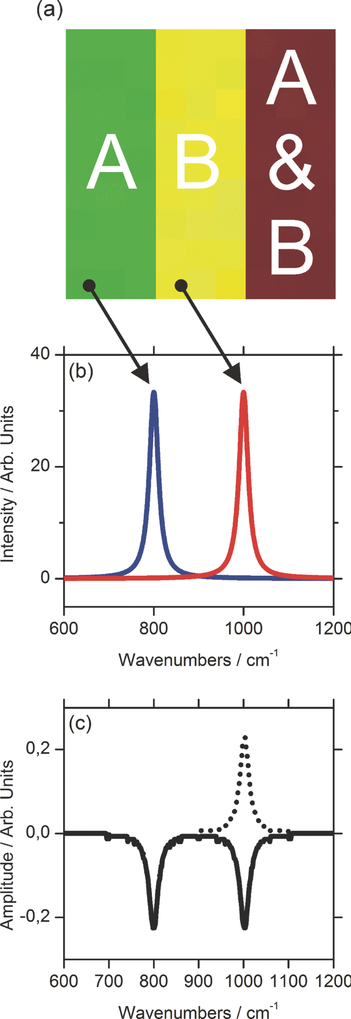

The first two eigenvectors required for fitting the different sample areas are shown in Fig. 4c, offering an important aspect of the PCA-method. They cannot be directly compared to the spectrum of each chemical component. For example, component A requires a linear combination of both eigenvectors with negative scaling factors. It follows that using the RGB imaging procedure, negative EVAs also have to be taken into account when designating the different colors.

In order to evaluate the sensitivity and the detection limits of our method, we investigated the influence of the line width, the distance between lines as well as the intensity (concentration squared). In order to quantify the sensitivity, we defined the color-contrast between the first sample area with component A and the third sample area containing both components A and B [Fig. 4a]. This way, it is possible, for a fixed concentration of component A, to quantify the concentration effect of component B on the parameters cited above. Note that the EVAs have been scaled between 0 and 255 for color coding. By subtracting the average EVA value of the first and second eigenvector on each sample area, it is possible to define a figure of merit for the color-contrast

Since the maximum value for an EVA is 255, the maximum theoretical value (510) for the color-contrast is obtained when, for example, the component A and B is fully described by just one eigenvector each. However, as already discussed above, a chemical component can be a linear superposition of the main eigenvectors, resulting in a color-contrast much lower than the maximum possible numerical value.

Figure 5a shows the image contrast dependence on the concentration of B for several line separations rising from 10 to 200 cm⁻¹. In general, the highest value of contrast is obtained when the concentrations (and therefore, spectral intensity) of A and B are similar, as one would expect. The plot also shows that reasonable image contrast can be obtained until the concentration of B drops below about 30%, which corresponds to a signal intensity of less than 10% from the original value. The dependence of the color-contrast on the Raman line separation is more intricate. Figure 5a challenges the usual assumption that well separated lines should generate the best color-contrast. The contrast obtained with the PCA analysis is determined by the scaling and overlapping between the eigenvectors, resulting in nontrivial dependence. For example, at a concentration for component B of about 75%, a Raman line separation of 10 cm⁻¹ results in a high contrast; this contrast then initially decreases when the lines are 50 cm⁻¹ apart and increases again when the lines are more separated. Nevertheless, the principal component analysis results in a high image contrast even when Raman lines are well superimposed.

Fig. 5

(a) Contrast at several line separations of A and B dependent on the concentration of B. The distances are 200 cm⁻¹ (inverted triangles), 100 cm⁻¹ (triangles), 50 cm⁻¹ (circle), 25 cm⁻¹ (diamonds), and 10 cm⁻¹ (square). Line width of component A and B was kept constant with 24 cm⁻¹. Contrast decreases with the concentration of component B. (b) Experimental dilution series of toluene in cyclohexane with linear fit in the log scale and a slope of 2.1.

It is interesting to consider whether the lower limit for the sensitivity constrains the overall sensitivity of the MCARS experiment. In order to test it, in our MCARS setup we experimentally measured the concentration of toluene in cyclohexane and plotted the ratio of two lines of each component in Fig. 5b. We were able to experimentally detect toluene concentrations as low as 20%. In short, the detection limit of the data analysis is fairly similar to the experimental detection limit of our MCARS setup.

The influence of the line width of component B on the sensitivity of the EVA-method is shown in Fig. 6a for a fixed line separation of 200 cm⁻¹. The intensity of the spectrum of the component B was rescaled accordingly in order to keep A and B with the same amplitude. It is clear to observe the improvement of the image contrast for an increasing line width of component B. This diagram also points out the detection limit concerning the line width of the Raman line: At least 6 cm⁻¹ (FWHM) can be properly discriminated, what is definitely under the experimental resolution of about 16 cm⁻¹. The best contrast is obtained when component A and B have the same FWHM. Since for the PCA analysis the FWHM of component A and B is a symmetrical problem and the relative value is the important factor, when the line width of component B increases compared to the line width of component A (FWHM_[B] > FWHM_[A]), the image contrast decreases accordingly.

In Fig. 6b, the line width of the Raman lines of both components is kept constant whereas the line separation is changed. In Fig. 6, it is important to notice that the signal intensity of component B was kept at 10% of component A, a value below the detection limit described above. For smaller distances, the contrast increases one order of magnitude until the line separation has reached the theoretical value of 0 cm⁻¹. This value can also be obtained at a larger distance (black bar) when the intensity of A is increased to 110% of its initial value when it appears in the presence of B. In other words, the improved contrast is based on increased signal intensity of A by positive interference with B. Such a result can be explored later, for example, to improve color-contrast by using external overlapping Raman bands.

Fig. 6

(a) The contrast improves for increasing FWHM of component B. The line separation is 200 cm⁻¹, intensity of B is fixed at 100% of A. Line width of component A was kept constant with 24 cm⁻¹. (b) Contrast while B is set at 10% intensity of A at several distances. The increased contrast in case of small distances is caused by positive interference between A and B. Additional 10% of intensity to A in field 3 [see Fig. 4b] has the same effect as the addition of B to A (black bar).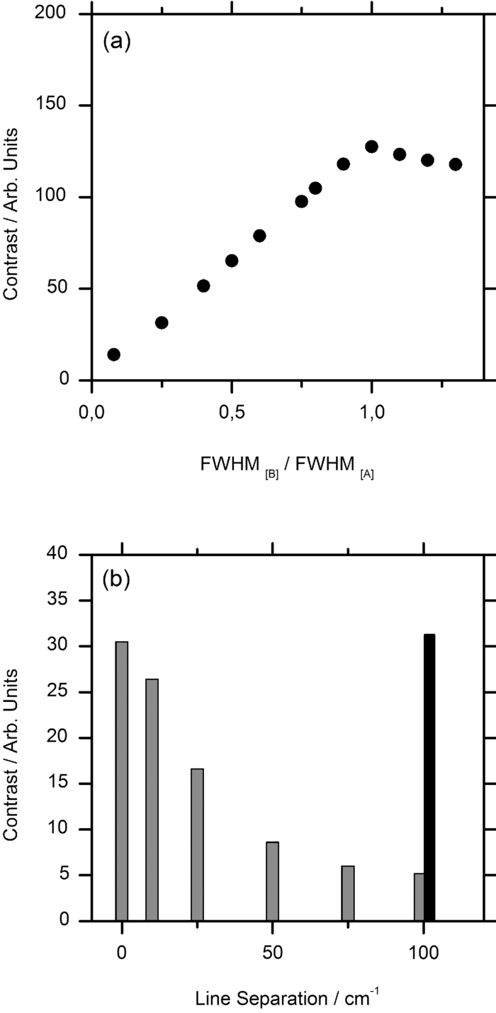

5.

Application to Polymer and Biological Samples

The image processing program described thus far was finally applied to polymeric and biological samples in order to show its capability in chemical imaging. The polymer system was especially designed for our MCARS studies. A strong Raman active media such as diiodobenzene was encapsulated in polyamide resulting in polymer microcapsules measuring several micrometers in diameter. Therefore, the MCARS spectra recorded from the shell should differ from the core and be distinguished by our imaging algorithm. In Fig. 7a, the brightfield image of the polymer microcapsules is shown. Round structures can be identified without any reference to a binary structure or to the two different chemical components. The result dramatically changes when the picture is taken by MCARS microscopy and analyzed with our fitting algorithm [Fig. 7b]. By plotting the eigenvector amplitudes from the highest valued eigenvectors 1–3, the inner spheres of the capsules appear in red clearly surrounded by the shells appearing in green. The third component shown in blue primary belongs to the nonresonant background. It shows up mainly in the empty spaces between the capsules, where neither the polymer nor the diiodobenzene can be found. The weak contribution of the third component, resulting in a dark color directly indicates weak signal intensity compared to the sample components.

Fig. 7

(a) Brightfield image of polymer microcapsules. (b) The MCARS image analyzed with imaginary part extraction and PCA. (c) MCARS image analyzed using single Raman spectral features (CH-vibration at 2912 cm⁻¹, CH-vibration at 2912 cm⁻¹, and vibration at 1777 cm⁻¹). (d) MCARS image analyzed only with PCA.

In Fig. 8, a spectrum taken from the core is compared with a spectrum taken from the shell. Besides a more pronounced region of unsaturated CH-stretching vibrations as discussed above, there are several differences in lineshape and intensity. The important point is that these differences are very small and spread over the whole spectral region. This observation originates from the lack of sharp spectral features in the signal of p-diiodobenzene combined with reduced spatial resolution in the z-direction. In spite of that, our two-step approach is already able to extract the spectral information necessary to provide Fig. 7b. The result shown in Fig. 7b could not be obtained by taking the amplitude of a single spectral feature for image contrast as performed by traditional analysis.^{34, 35, 36} This can be unmistakably observed by comparing Figs. 7b and 7c. If we take into account the amplitude of the three main Raman lines at 3064 cm⁻¹, 2912 cm⁻¹, and 1777 cm⁻¹ and associate three different colors to each mode, respectively [Fig. 7c], we are still unable to reproduce the shell structure nicely distinguished with our method [Fig. 7b].

Fig. 8

Reconstructed Raman spectrum of microcapsules core (red) and shell (green). Several small spectral differences are diluted over the whole spectral region. Inset: Spectral region between 1000 cm⁻¹ and 2000 cm⁻¹. Signals are vertically displaced for better visualization.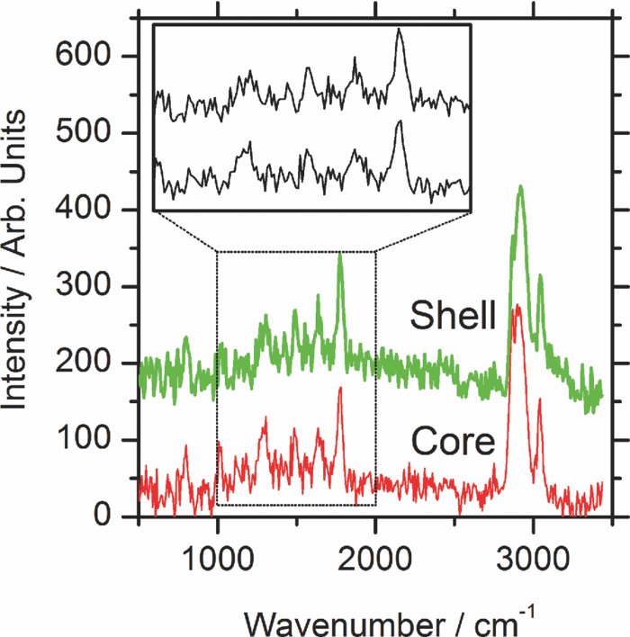

The remaining question at this point is the influence of the fitting algorithm that precedes the PCA and extracts the spontaneous Raman data. A fourth result based only on the MCARS raw data combined with PCA is shown in Fig. 7d. Although the coarse structure of the sample is clearly separated from the background, it was not possible to reproduce the shell, no matter which combination of eigenvectors has been chosen. This result unquestionably shows that real spectral differences are responsible for the result in Fig. 7b and that it is not caused by secondary effects, such as light guiding in the case of spherical and transparent polymer particles.

Furthermore, Fig. 9 offers an additional aspect regarding the importance of imaginary part extraction when combined with PCA. Based on the covariance matrix of the polymer sample, eigenvectors one and two are shown using the raw data and the fitting algorithm from Liu ²⁸ For example, the features around 3000 cm⁻¹ dramatically change when the dispersive line profile of the raw data is corrected. The role of phase retrieval can be quantified in the variance of each eigenvector: The relative variance of the first eigenvector is lowered from 98% to 54% whereas the variance of the second eigenvector rises from 1% to 2%. Imaginary part extraction, therefore, increases the amount of information represented by the second eigenvector. The previous fitting algorithm corrects the destructive interferences blue shifted to strong vibrational modes. This can be considered as an improvement of signal to background ratio of weak MCARS signals.

Fig. 9

(a) Eigenvector 1 of the polymer sample obtained with imaginary part extraction (red line) and without (black line). (b) Analogous plot as in (a) for eigenvector 2.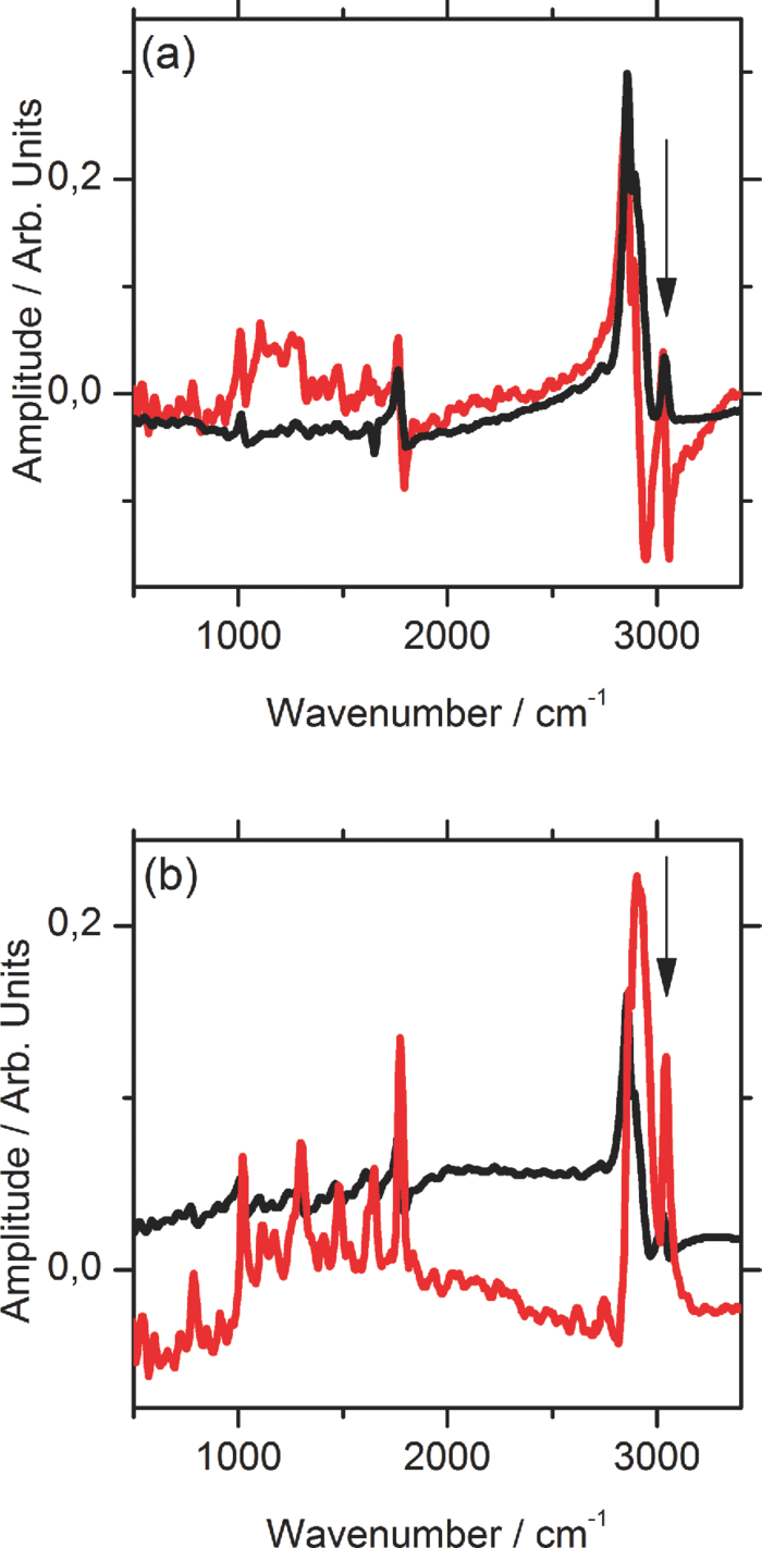

The second example focuses on living cells of plants, namely the moss Plagiomnium rostratum, as an example of small biological structures combined with weak signal intensities. A juvenile leaf of a fast growing species was prepared on a microscope slide and a cover slip to prevent desiccation. The brightfield image is shown in Fig. 10a and was recorded in the same manner as in Fig. 7a. The typical hexagonal morphology of the cells can be clearly observed but detailed intracellular morphological substructure cannot be identified due to the mostly transparent sample. In contrast, the MCARS image analyzed with our fitting algorithm [Fig. 10b] resolves the cellular structures in a brilliant manner, unambiguously uncovering chemical details of the main biological components hidden from brightfield microscopy. For example, in Figs. 10c, 10d, 10e we are able to identify three structures. The intercellular area (“framework”), marked with the green color, has a spectrum with a pronounced contribution at 2900 cm⁻¹, which can be identified as cellulose with its typical CH-stretching mode [Fig. 10c]. Regions marked with the red color have a very structured spectrum, with a vibrational mode at about 1500 cm⁻¹ and a broad band originated from two-photon fluorescence (located at about 2000 cm⁻¹). ^{37, 38} These spectral features have been discussed in other experiments to be originated by chlorophyll, which leads us to identify the red-marked structures as the chloroplasts. It can be nicely observed that the chloroplasts, as key structures in photosynthesis, are localized at the inner walls of the cells with a dimension around 2–4 μm [Fig. 10d]. The remaining region [Fig. 10e], which is identified as vacuoles and lacks in general a structured Raman spectrum, is mainly found inside the cells and is shown as a round dark blue structure surrounded by the chloroplasts. Moreover, additional CH-stretching vibration signals at the inside of the cells indicate further biological components, e.g., the core and Golgi apparatus, and show up as a mixed color between the green and blue parts leading to a light blue color. These results show that our analysis method is an excellent tool for the noninvasive examination of living cells, especially concerning the localization of cell organelles exemplified here in the case of plant cells.

Fig. 10

(a) Brightfield image of living cells of Plagiomnium rostratum. (b) The MCARS image using MCARS data valuated with imaginary part extraction and PCA. (c)–(e) Reconstructed Raman spectra of each biological component. Residual disturbed line profiles in the reconstructed Raman spectra are due to intense 2-photon fluorescence of the chlorophyll and the strong nonresonant background. Additional baseline subtraction was performed to suppress strong fluorescence contribution. See text for discussion.

6.

Conclusion and Outlook

The nonbiased analysis of complex imaging data obtained with CARS techniques has been a long standing goal in the nonlinear microscopy. In this work we have successfully developed a new approach to generate chemoselective images of CARS signals. By combining a global fitting procedure based on principal component analysis with the imaginary part extraction of the CARS signal, we have shown that the whole complex Raman spectrum can be used to clearly distinguish (bio-) chemical components of a completely unknown sample. Such a two-step signal analysis scheme is essential in automatically obtaining chemoselective image contrast without any a priori chemical information on the sample. The fitting results are available within a few minutes using a standard desktop computer but should be easily improved by a state-of-the-art computer. In contrast to previous approaches, where only one spectral feature of the CARS signal is taken in account, here we have shown that small differences spread over the whole Raman spectrum must be considered in order to achieve optimal chemical separation of similar components. This analysis method was successfully tested in a specially designed sample containing polymer microcapsules as well as in living cells of plants as a highly structured biological sample.

Last but not least, our two-step method can be further improved regarding quantitative information and determination of the pure spectra by using, for example, other approaches to extract the imaginary part of the CARS signal such as the maximum entropy methods or different types of global fitting routines such as cluster analysis, functional PCA, or artificial neuronal networks. We believe that in the future the procedure introduced here will help to improve CARS microscopy in live sciences, particularly in the analysis of complex biological tissues where several chemical components overlap.