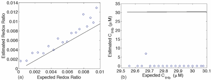
1.

Introduction

Quantitative spectroscopic imaging techniques for medical diagnostics have become a hot research area in past decades. In particular, the reduction-oxidation (redox) ratio in tissues is an important metabolic biomarker valuable in both biological science research and clinical diagnostics. Fluorescence spectroscopy has been used to estimate the redox ratio in a wide variety of applications other than brain cancer diagnoses. The estimation of the redox ratio involves the measurement of fluorescence intensities of two fluorophores, reduced nicotinamide adenine dinucleotide (NADH), and flavin adenine dinucleotide (FAD). The definition of the redox ratio is not always consistent in the literature. Skala et al.¹ employed two-photon microscopy to measure the fluorescence redox ratio, which was defined as the ratio of the fluorescence intensity of FAD and that of NADH in this study, in a dimethylbenzanthracene (DMBA)-treated hamster cheek pouch model of oral cancer. It was found that the redox ratio was significantly lower in the less differentiated basal epithelial cells than the more mature cells in the superficial layer of the normal stratified squamous epithelium. However, the same trend was not observed in the superficial and basal cells of precancerous tissues. Ranji et al.² used in vivo fluorescence spectroscopy and imaging to study redox ratio change in myocardial apoptosis, in which the redox ratio was defined as the ratio of the fluorescence intensity of FAD and the sum of the fluorescence intensities of FAD and NADH. The higher redox ratios measured in vivo and in snap-frozen hearts were both correlated with the initiation of apoptosis following heart reperfusion. Drezek et al.³ assessed the differences in autofluorescence of fresh tissue sections between normal and dysplastic cervical tissues, in which the redox ratio was also defined as the ratio of the fluorescence intensity of FAD and the sum of the fluorescence intensities of FAD and NADH. A decreased redox ratio in dysplastic tissue sections was observed in one-third of the paired samples, which indicates increased metabolic activity. The sources of autofluorescence were confirmed by a laser-induced fluorescence study using confocal microscopy⁴ to be mitochondrial NADH and FAD when the excitation wavelength was 351–364 nm and 488 nm, respectively.

The studies in the redox state of brain tumors as opposed to normal brain tissues are relatively less reported despite many publications about the use of fluorescence spectroscopy for brain cancer diagnostics. Chung et al.⁵ measured two-dimensional excitation and emission matrices of in vitro human brain tissues under a fiber-optic probe geometry. It was found that both NAD(P)H and flavin fluorescence were lower in all measured human brain tumors than in normal brain tissues, but the ratio of NADH to Flavin fluorescence was not significantly different between them. Light absorption that was not removed likely blurred the difference in fluorescence spectra between tumors and normal tissues. Lin et al.⁶ explored the use of combined fluorescence and diffuse reflectance spectroscopy for in vivo brain tumor demarcation and reported excellent accuracy (a sensitivity of 100% and a specificity of 76%). However, because only one excitation wavelength (337 nm) was used to excite NADH fluorescence, there was no derivation of redox ratios attempted. Croce ⁷ investigated the autofluorescence properties of nonneoplastic and neoplastic brain tissues in tissue sections and homogenates by use of a microspectrofluorometer, and directly on patients affected by glioblastoma multiforme during surgery with a fiber-optic probe. They used a ratio of fluorescence intensities at 520 and 470 nm for an excitation wavelength of 405 nm to characterize the change in the spectral shape with neoplastic growth. It was found that the ratio in neoplastic tissue is higher than that in non-neoplastic tissue. However, their results were not true redox ratios because the fluorescence from different fluorophores was not separated in the calculation of ratios. Lin ⁸ used three excitation wavelengths, 337, 360, and 440 nm to differentiate pediatric neoplastic and epileptogenic brain from normal brain and found statistically significant differences between neoplastic brain and normal gray/white matters. However, they did not report the results of redox ratio because the effect of light absorption on fluorescence spectra was not removed in this study. Mayevsky and Chance⁹ have shown that by subtracting the reflectance signal from the fluorescence signal in 1:1 ratio, the effect of hemoglobin is significantly diminished. However, the optimal wavelengths and the effect of illumination and detection configuration were not discussed. Zhang et al.¹⁰ investigated the use of fluorescence redox ratio as an indicator for the response of photodynamic therapy (PDT) of a 9L-glioma-bearing rat model using an imaging configuration. After a glioma was treated by PDT, its redox ratio, which was again defined as the ratio of the fluorescence intensity of FAD and the sum of the fluorescence intensities from FAD and NADH, increased suggesting that the redox ratio is a nice indicator for measuring PDT-induced tissue damage.

Although fluorescence measured from thin tissue sections in various microscopic techniques, such as multiphoton microscopy, is usually free of distortion from light absorption primarily due to hemoglobin, fluorescence spectra measured from a large tissue volume by a fiber-optic probe geometry or an imaging geometry are subject to hemoglobin absorption in general. The redox ratio calculated from these fluorescence spectra may not faithfully represent the true metabolic condition. This is a challenge frequently encountered in many in vivo fluorescence spectroscopy studies.

Several methods¹¹ have been developed to extract intrinsic fluorescence spectra that are free of distortion from tissue absorption from raw spectra. However, many of these methods^{12, 13, 14} are designed for extracting fluorescence spectra, which requires all the raw fluorescence spectra and typically involves fitting data to a complicated light transport model by applying nonlinear regression. The computational load for these methods can be high, thus, are often not suitable for real time tissue monitoring in a large field of view, for example, in tumor-margin assessment during brain surgery. Some groups proposed ratiometric methods that could reduce the complexity of computation. Avrillier et al.¹⁵ have modeled the medium function using a semianalytical Monte Carlo method and taken the ratio of measured fluorescence to the medium function to cancel out the effect of tissue turbidity on fluorescence spectra, which requires a separate measurement of the medium function thus is not practical for real-time applications. Kramer and Pearlstein¹⁶ took the ratio of measured NADH fluorescence at two isosbestic wavelengths to prevent the variation of a single measurement with hemoglobin oxygenation, but the effect of total hemoglobin was still present. Several other groups^{17, 18, 19, 20} reported using the ratio of fluorescence and diffuse reflectance or the variants of the ratio to correct for the effect of tissue absorption and scattering and obtain intrinsic fluorescence (see Ref. 11 for a more comprehensive review about this technique). This would require an additional optical module for diffuse reflectance measurements.

We have proposed a ratiometric method previously²¹ based on the spectral filtering modulation of fluorescence spectra for the estimation of hemoglobin concentration and oxygenation using only a few data points in a fluorescence emission spectrum. Because our method directly uses fluorescence data to obtain hemoglobin information, it does not require separate equipment or measurement procedures for diffuse reflectance measurements. This method does not need to fit the spectrum to complicated mathematical light transport models, thus, greatly reducing the computational load. The ratiometric nature of this method makes it resistant to the variation in optical coupling. Simple calibration curves were established for estimating total hemoglobin concentration and oxygen saturation.

In this paper, we extend the spectral filtering modulation method to estimate the intrinsic fluorescence redox ratio based on fluorescence intensities at only three wavelengths. Because only a few data points in one single fluorescence emission spectrum are required to derive intrinsic fluorescence redox ratio, there is no need to calibrate the wavelength dependence of system throughput and data acquistion and analysis can be performed rapidly. The principle of this method and the validation in phantom experiments are briefly described. The effect of emission wavelengths and fiber-optic probe geometry are discussed. The method was applied in an orthotopic intracranial brain tumor model in the rat to measure redox ratios in both normal tissues and tumors. The trend in the change of redox ratio from normal tissues to tumors agrees with previously published studies. The limitations and potential advantages of the method will be discussed.

2.

Materials and Methods

2.1.

Spectral Filtering Modulation Method for Estimation of Intrinsic Fluorescence Redox Ratio

We have previously developed a spectral filtering modulation method²¹ to extract hemoglobin concentration and oxygenation from a few data points in a fluorescence emission spectrum. This method assumes a homogeneous tissue model that contains hemoglobin as the major absorber and a single-known major fluorophore. Furthermore, the excitation wavelength is close to the absorption peak of hemoglobin and the emission wavelength is far from the absorption peak; thus, the absorption coefficient at the emission wavelength is much weaker than that at the excitation wavelength.

The fluorescence measured from a turbid tissue model can be expressed as

Eq. 1

[TeX:] \documentclass[12pt]{minimal}\begin{document}\begin{equation} F_{{\rm Measured}} \propto F_{{\rm Intrinsic}} e^{ - \mu _{{\rm a\_m}} \left\langle l \right\rangle }, \end{equation}\end{document} $$F_{\mathrm{Measured}}\propto F_{\mathrm{Intrinsic}}{e}^{-{\mu }_{\mathrm{a}\_\mathrm{m}}〈l〉},$$

where F _Measured is measured fluorescence, F _Intrinsic is the intrinsic fluorescence of the tissue model in which the effects of absorption and scattering have been removed, μ_{a_m} is the absorption coefficient of the tissue model at the emission wavelength and 〈l〉 is the average emission path length of detected fluorescence photons. It should be noted that all quantities are a function of the fluorescence emission wavelength. Equation 1 is valid when the distribution of 〈l〉 is centered on the average value with a small deviation. The distribution of 〈l〉 is determined by the scattering properties of the tissue model at both the excitation and emission wavelengths.

The ratio of fluorescence intensities at two emission wavelengths is

Eq. 2

[TeX:] \documentclass[12pt]{minimal}\begin{document}\begin{equation} \frac{{F_{{\rm Measured\_1}} }}{{F_{{\rm Measured\_2}} }} \approx \frac{{F_{{\rm Intrinsic\_1}} }}{{F_{{\rm Intrinsic\_2}} }}e^{ - \left({\mu _{{\rm a\_m1}} - \mu _{{\rm a\_m2}} } \right)\left\langle l \right\rangle }, \end{equation}\end{document} $$\frac{F_{\mathrm{Measured}\_1}}{F_{\mathrm{Measured}\_2}}\approx \frac{F_{\mathrm{Intrinsic}\_1}}{F_{\mathrm{Intrinsic}\_2}}{e}^{-\left({\mu }_{\mathrm{a}\_\mathrm{m}1}-{\mu }_{\mathrm{a}\_\mathrm{m}2}\right)〈l〉},$$

where the subscripts 1 and 2 indicate two emission wavelengths λ₁ and λ₂. The two wavelengths should be close enough such that 〈l〉 at two wavelengths can be assumed equal. The previous finding,²² that tissue scattering changes slowly with light wavelength, would also help meet this assumption.

This method can be extended to accommodate the case of multiple fluorophores. Assume that hemoglobin is the major absorber in the tissue model and the intrinsic fluorescence contributed by each fluorophore is proportional to its concentration. Then the difference in the absorption coefficients in the exponent term of Eq. 2 can be written in terms of hemoglobin concentration and oxygenation,²¹ Furthermore, the two intrinsic fluorescence terms can be expressed as the linear summation of contributions from individual fluorophores. Equation 2 becomes

Eq. 3

[TeX:] \documentclass[12pt]{minimal}\begin{document}\begin{equation} \frac{{F_{{\rm Measured\_1}} }}{{F_{{\rm Measured\_2}} }} \approx \frac{{\sum\limits_{i = 1}^N {C_i \phi _{i\_1} } }}{{\sum\limits_{i = 1}^N {C_i \phi _{i\_2} } }}e^{ - \left[ {C_{{\rm tHb}} (\varepsilon _{{\rm Hb\_1}} - \varepsilon _{{\rm Hb\_2}}) + C_{{\rm tHb}} {\rm StO}_2 (\Delta \varepsilon _1 - \Delta \varepsilon _2)} \right]\left\langle l \right\rangle }, \end{equation}\end{document} $$\frac{F_{\mathrm{Measured}\_1}}{F_{\mathrm{Measured}\_2}}\approx \frac{\sum _{i=1}^N{C}_i{\phi }_{i\_1}}{\sum _{i=1}^N{C}_i{\phi }_{i\_2}}{e}^{-\left[C_{\mathrm{tHb}}({\varepsilon }_{\mathrm{Hb}\_1}-{\varepsilon }_{\mathrm{Hb}\_2})+C_{\mathrm{tHb}}{\mathrm{StO}}_2(\Delta {\varepsilon }_1-\Delta {\varepsilon }_2)\right]〈l〉},$$

where N is the total number of different fluorophores in the tissue model, ϕ_i and C _i are the quantum yield and concentration of the i‘th fluorophore, respectively, C _tHb is the total hemoglobin concentration regardless of oxygenation, StO₂ is hemoglobin oxygenation, ɛ_Hb and [TeX:] $\varepsilon _{{\rm Hb\_O}_{\rm 2} }$ ${\varepsilon }_{{\mathrm{Hb}\_\mathrm{O}}_2}$ are the molar extinction coefficients of deoxygenated hemoglobin and oxygenated hemoglobin, respectively. Moreover, [TeX:] $\Delta \varepsilon _1 = \varepsilon _{{\rm HbO}_{\rm 2} {\rm \_1}} - \varepsilon _{{\rm Hb\_1}}$ $\Delta {\varepsilon }_1={\varepsilon }_{{\mathrm{HbO}}_2\_1}-{\varepsilon }_{\mathrm{Hb}\_1}$ , [TeX:] $\Delta \varepsilon _2 = \varepsilon _{{\rm HbO}_{\rm 2} {\rm \_2}} - \varepsilon _{{\rm Hb\_2}}$ $\Delta {\varepsilon }_2={\varepsilon }_{{\mathrm{HbO}}_2\_2}-{\varepsilon }_{\mathrm{Hb}\_2}$ .

Taking the logarithm of Eq. 3 yields

Eq. 4

[TeX:] \documentclass[12pt]{minimal}\begin{document}\begin{eqnarray} &&\hspace*{-10pt}\log \frac{{F_{{\rm Measured\_1}} }}{{F_{{\rm Measured\_2}} }} \approx \log \left({\frac{{\sum\limits_{i = 1}^N {C_i \phi _{i\_1} } }}{{\sum\limits_{i = 1}^N {C_i \phi _{i\_2} } }}} \right)\nonumber\\ &-& \left[ {C_{{\rm tHb}} (\varepsilon _{{\rm Hb\_1}} - \varepsilon _{{\rm Hb\_2}}) + C_{{\rm tHb}} {\rm StO}_2 (\Delta \varepsilon _1 - \Delta \varepsilon _2)} \right]\left\langle l \right\rangle. \end{eqnarray}\end{document} $$\begin{array}{ccc}& & \log \frac{F_{\mathrm{Measured}\_1}}{F_{\mathrm{Measured}\_2}}\approx \log \left(\frac{\sum _{i=1}^N{C}_i{\phi }_{i\_1}}{\sum _{i=1}^N{C}_i{\phi }_{i\_2}}\right)\hfill \\ & -& \left[C_{\mathrm{tHb}}({\varepsilon }_{\mathrm{Hb}\_1}-{\varepsilon }_{\mathrm{Hb}\_2})+C_{\mathrm{tHb}}{\mathrm{StO}}_2(\Delta {\varepsilon }_1-\Delta {\varepsilon }_2)\right]〈l〉.\hfill \end{array}$$

If λ₁ and λ₂ are chosen to be the isosbestic wavelengths of hemoglobin absorption such that [TeX:] $\varepsilon _{{\rm Hb\_1}} = \varepsilon _{{\rm HbO}_{\rm 2} {\rm \_1}}$ ${\varepsilon }_{\mathrm{Hb}\_1}={\varepsilon }_{{\mathrm{HbO}}_2\_1}$ and [TeX:] $\varepsilon _{{\rm Hb\_2}} = \varepsilon _{{\rm HbO}_{\rm 2} {\rm \_2}}$ ${\varepsilon }_{\mathrm{Hb}\_2}={\varepsilon }_{{\mathrm{HbO}}_2\_2}$ , Eq. 4 will be reduced to

Eq. 5

[TeX:] \documentclass[12pt]{minimal}\begin{document}\begin{equation} \log \frac{{F_{{\rm Measured\_1}} }}{{F_{{\rm Measured\_2}} }} \approx \log \left({\frac{{\sum\limits_{i = 1}^N {C_i \phi _{i\_1} } }}{{\sum\limits_{i = 1}^N {C_i \phi _{i\_2} } }}} \right) - C_{{\rm tHb}} (\varepsilon _{{\rm Hb\_1}} - \varepsilon _{{\rm Hb\_2}})\left\langle l \right\rangle. \end{equation}\end{document} $$\log \frac{F_{\mathrm{Measured}\_1}}{F_{\mathrm{Measured}\_2}}\approx \log \left(\frac{\sum _{i=1}^N{C}_i{\phi }_{i\_1}}{\sum _{i=1}^N{C}_i{\phi }_{i\_2}}\right)-C_{\mathrm{tHb}}({\varepsilon }_{\mathrm{Hb}\_1}-{\varepsilon }_{\mathrm{Hb}\_2})〈l〉.$$

For certain illumination-detection configurations, the parameter 〈l〉 at two emission wavelengths can be approximated as equal and remain roughly at a constant in the target tissue model. When 〈l〉 is small enough such that the second term on the right-hand side of Eq. 5 is ≪1, Eq. 5 can be simplified by applying the exponential operation and then performing the first-order Taylor expansion, i.e.,

Eq. 6

[TeX:] \documentclass[12pt]{minimal}\begin{document}\begin{equation} \frac{{F_{{\rm Measured\_1}} }}{{F_{{\rm Measured\_2}} }} \approx \frac{{\sum\limits_{i = 1}^N {C_i \phi _{i\_1} } }}{{\sum\limits_{i = 1}^N {C_i \phi _{i\_2} } }}\left[ {1 - C_{{\rm tHb}} (\varepsilon _{{\rm Hb\_1}} - \varepsilon _{{\rm Hb\_2}})\left\langle l \right\rangle } \right]. \end{equation}\end{document} $$\frac{F_{\mathrm{Measured}\_1}}{F_{\mathrm{Measured}\_2}}\approx \frac{\sum _{i=1}^N{C}_i{\phi }_{i\_1}}{\sum _{i=1}^N{C}_i{\phi }_{i\_2}}\left[1-C_{\mathrm{tHb}}({\varepsilon }_{\mathrm{Hb}\_1}-{\varepsilon }_{\mathrm{Hb}\_2})〈l〉\right].$$

Rearranging terms yields

Eq. 7

[TeX:] \documentclass[12pt]{minimal}\begin{document}\begin{equation} \frac{{{{F_{{\rm Measured\_1}} } \mathord{\left/ {\vphantom {{F_{{\rm Measured\_1}} } {F_{{\rm Measured\_2}} }}} \right. \kern-\nulldelimiterspace} {F_{{\rm Measured\_2}} }}}}{{{{\sum\limits_{i = 1}^N {C_i \phi _{i\_1} } } \mathord{\left/ {\vphantom {{\sum\limits_{i = 1}^N {C_i \phi _{i\_1} } } {\sum\limits_{i = 1}^N {C_i \phi _{i\_2} } }}} \right. \kern-\nulldelimiterspace} {\sum\limits_{i = 1}^N {C_i \phi _{i\_2} } }}}} \approx 1 - C_{{\rm tHb}} (\varepsilon _{{\rm Hb\_1}} - \varepsilon _{{\rm Hb\_2}})\left\langle l \right\rangle. \end{equation}\end{document} $$\frac{F_{\mathrm{Measured}\_1}/\phantom{F_{\mathrm{Measured}\_1}{F}_{\mathrm{Measured}\_2}}{F}_{\mathrm{Measured}\_2}}{\sum _{i=1}^N{C}_i{\phi }_{i\_1}/\phantom{\sum _{i=1}^N{C}_i{\phi }_{i\_1}\sum _{i=1}^N{C}_i{\phi }_{i\_2}}\sum _{i=1}^N{C}_i{\phi }_{i\_2}}\approx 1-C_{\mathrm{tHb}}({\varepsilon }_{\mathrm{Hb}\_1}-{\varepsilon }_{\mathrm{Hb}\_2})〈l〉.$$

The left-hand side of Eq. 7 is named the attenuation ratio because it represents the attenuation in the fluorescence ratio due to hemoglobin absorption. The attenuation ratio is linearly proportional to total hemoglobin concentration to the first-order approximation. Thus, Eq. 7 represents a simple empirical method for estimating both the concentrations of fluorophores C _i and total hemoglobin concentration C _tHb. This method can be formulated in two steps, i.e., the calibration step and the measurement step.

First, a calibration procedure is carried out to determine the relationship between the attenuation ratio and C_tHb as in Eq. 7. For this purpose, a series of tissue phantoms will be made in which only a single fluorophore is present and total hemoglobin concentration is varied to cover a representative range of the absorption coefficient in human epithelial tissue.²³ Because there is only one fluorophore, the denominator on the left-hand side of Eq. 7 is reduced to ϕ₁/ϕ₂, which can be easily derived from the fluorescence spectrum of an optically dilute phantom that contains only the fluorophore. After fluorescence spectra are measured from all phantoms, the attenuation ratio on the left-hand side of Eq. 7 will be calculated and a system of linear equations will be fit to Eq. 7 to find the relation. The result of the calibration procedure is shown in Fig. 3. It should be noted that the concentration of the single fluorophore in calibration phantoms should be sufficiently low so that the absorption coefficient contributed by the fluorophore is negligible compared to that by hemoglobin.

Fig. 3

Calibration curves for estimating total hemoglobin concentration: (a) F500nm/F545nm; (b) F500nm/F570nm. The calibration curves were the attenuation ratio as a function of total hemoglobin concentration. The attenuation ratio is calculated by dividing the fluorescence ratio measured from the turbid phantom by the fluorescence ratio measured from the corresponding optically dilute phantom that contained FAD only. The data points with the legend “Average” are the average of the attenuation ratios for all three scattering coefficients and the corresponding linear fittings are labeled as “linear” in the legend.

Second, fluorescence ratios are calculated from fluorescence spectra of tissue samples in which multiple known fluorophores are present. The intrinsic fluorescence spectrum of each fluorophore can be measured beforehand. In a tissue model with N fluorophores, N fluorescence ratios are required. These fluorescence ratios will be fit to Eq. 7 in order to find the ratio of fluorophore concentrations C _i/C₁, i = 1,…,N−1, and total hemoglobin concentration C _tHb, where C ₁ can be the concentration of any fluorophore in the tissue model. It is noted that this approach naturally yields concentration ratios thus suitable for the redox ratio analysis.

Because the fluorescence redox ratio involves two fluorophores (i.e., NADH and FAD), two fluorescence ratios are required to derive the redox ratio and hemoglobin concentration. In this study, the following three wavelengths, 500, 545, and 570 nm, were chosen to generate two fluorescence ratios for the estimation of the redox ratio. These three wavelengths are the isosbestic wavelengths of hemoglobin absorption; furthermore, both NADH and FAD exhibit considerable fluorescence at each wavelength. In addition, they are close to each other, which is necessary to meet the assumption of equal average emission path lengths. Equation 8 shows the relation between the measured fluorescence ratio and the concentration ratio of NADH and FAD, in which [NADH]/[FAD] is the molar concentration ratio of NADH and FAD, ϕ represents the fluorescence quantum yield for the specified fluorophore and wavelength, a and b are the intercept and slope of the calibration line for atteunatio ratios established in the calibration step at the specified wavelength. The calibration lines for two wavelength pairs [i.e., (500 nm, 545 nm) and (500 nm, 570 nm)], are shown in Fig. 3,

Eq. 8

[TeX:] \documentclass[12pt]{minimal}\begin{document}\begin{equation} \left\{ {\begin{array}{cc} \displaystyle{{{\left({\frac{{F_{{\rm Measured\_500}\,\,{\rm nm}} }}{{F_{{\rm Measured\_545}\,\,{\rm nm}} }}} \right)} \mathord{\left/ {\vphantom {{\left({\frac{{F_{{\rm Measured\_500}\,\,{\rm nm}} }}{{F_{{\rm Measured\_545}\,\,{\rm nm}} }}} \right)} {\left({\frac{{[{\rm NADH]/[FAD}] \bullet \phi _{{\rm NADH\_500}\,\,{\rm nm}} + \phi _{{\rm FAD\_500}\,\,{\rm nm}} }}{{[{\rm NADH]/[FAD}] \bullet \phi _{{\rm NADH\_545}\,\,{\rm nm}} + \phi _{{\rm FAD\_545}\,\,{\rm nm}} }}} \right)}}} \right. \kern-\nulldelimiterspace} {\left({\frac{{[{\rm NADH]/[FAD}] \bullet \phi _{{\rm NADH\_500}\,\,{\rm nm}} + \phi _{{\rm FAD\_500}\,\,{\rm nm}} }}{{[{\rm NADH]/[FAD}] \bullet \phi _{{\rm NADH\_545}\,\,{\rm nm}} + \phi _{{\rm FAD\_545}\,\,{\rm nm}} }}} \right)}} \approx a_{500/545} + C_{{\rm tHb}} b_{500/545} } \hfill \\[8pt] \displaystyle{{{\left({\frac{{F_{{\rm Measured\_500}\,\,{\rm nm}} }}{{F_{{\rm Measured\_570}\,\,{\rm nm}} }}} \right)} \mathord{\left/ {\vphantom {{\left({\frac{{F_{{\rm Measured\_500}\,\,{\rm nm}} }}{{F_{{\rm Measured\_570}\,\,{\rm nm}} }}} \right)} {\left({\frac{{[{\rm NADH]/[FAD}] \bullet \phi _{{\rm NADH\_500}\,\,{\rm nm}} + \phi _{{\rm FAD\_500}\,\,{\rm nm}} }}{{[{\rm NADH]/[FAD}] \bullet \phi _{{\rm NADH\_570}\,\,{\rm nm}} + \phi _{{\rm FAD\_570}\,\,{\rm nm}} }}} \right)}}} \right. \kern-\nulldelimiterspace} {\left({\frac{{[{\rm NADH]/[FAD}] \bullet \phi _{{\rm NADH\_500}\,\,{\rm nm}} + \phi _{{\rm FAD\_500}\,\,{\rm nm}} }}{{[{\rm NADH]/[FAD}] \bullet \phi _{{\rm NADH\_570}\,\,{\rm nm}} + \phi _{{\rm FAD\_570}\,\,{\rm nm}} }}} \right)}} \approx a_{500/570} + C_{{\rm tHb}} b_{500/570} } \hfill \\[-2pt] \end{array}} \right.. \end{equation}\end{document} $$\left\{\begin{array}{c}{\displaystyle \left(\frac{F_{\mathrm{Measured}\_500\mathrm{nm}}}{F_{\mathrm{Measured}\_545\mathrm{nm}}}\right)/\phantom{\left(\frac{F_{\mathrm{Measured}\_500\mathrm{nm}}}{F_{\mathrm{Measured}\_545\mathrm{nm}}}\right)\left(\frac{\left[\mathrm{NADH}]/[\mathrm{FAD}\right]•{\phi }_{\mathrm{NADH}\_500\mathrm{nm}}+{\phi }_{\mathrm{FAD}\_500\mathrm{nm}}}{\left[\mathrm{NADH}]/[\mathrm{FAD}\right]•{\phi }_{\mathrm{NADH}\_545\mathrm{nm}}+{\phi }_{\mathrm{FAD}\_545\mathrm{nm}}}\right)}\left(\frac{\left[\mathrm{NADH}]/[\mathrm{FAD}\right]•{\phi }_{\mathrm{NADH}\_500\mathrm{nm}}+{\phi }_{\mathrm{FAD}\_500\mathrm{nm}}}{\left[\mathrm{NADH}]/[\mathrm{FAD}\right]•{\phi }_{\mathrm{NADH}\_545\mathrm{nm}}+{\phi }_{\mathrm{FAD}\_545\mathrm{nm}}}\right)\approx a_{500/545}+C_{\mathrm{tHb}}{b}_{500/545}}\hfill \\ {\displaystyle \left(\frac{F_{\mathrm{Measured}\_500\mathrm{nm}}}{F_{\mathrm{Measured}\_570\mathrm{nm}}}\right)/\phantom{\left(\frac{F_{\mathrm{Measured}\_500\mathrm{nm}}}{F_{\mathrm{Measured}\_570\mathrm{nm}}}\right)\left(\frac{\left[\mathrm{NADH}]/[\mathrm{FAD}\right]•{\phi }_{\mathrm{NADH}\_500\mathrm{nm}}+{\phi }_{\mathrm{FAD}\_500\mathrm{nm}}}{\left[\mathrm{NADH}]/[\mathrm{FAD}\right]•{\phi }_{\mathrm{NADH}\_570\mathrm{nm}}+{\phi }_{\mathrm{FAD}\_570\mathrm{nm}}}\right)}\left(\frac{\left[\mathrm{NADH}]/[\mathrm{FAD}\right]•{\phi }_{\mathrm{NADH}\_500\mathrm{nm}}+{\phi }_{\mathrm{FAD}\_500\mathrm{nm}}}{\left[\mathrm{NADH}]/[\mathrm{FAD}\right]•{\phi }_{\mathrm{NADH}\_570\mathrm{nm}}+{\phi }_{\mathrm{FAD}\_570\mathrm{nm}}}\right)\approx a_{500/570}+C_{\mathrm{tHb}}{b}_{500/570}}\hfill \end{array}\right..$$

It can be seen that there are two unknowns (i.e., [NADH]/[FAD] and C _tHb) in Eq. 8 that can be easily solved. Because the redox ratio is typically defined as r = [FAD]/([FAD] + [NADH]), it can be derived from [NADH]/[FAD] by applying r = 1/(1 + [NADH]/[FAD]).

2.2.

Compact Point-Detection Fluorescence Spectroscopy System

To facilitate animal experiments, a portable fluorescence spectroscopy system was built and a fiber-optic probe was custom made by a company (C-Technologies, Inc., Bridgewater, New Jersey). Figures 1a and 1b show the schematics of the system and the probe configuration, respectively. A diode laser (Cube 405–50C, Coherent Inc., Santa Clara, California) generates laser light at 407 nm, which is delivered onto the sample through the excitation channel of the fiber-optic probe. The emission channel of the probe collects backscattered fluorescence light and sends it to a research-grade compact optical spectrometer (QE65000, Ocean Optics Inc., Dunedin, Florida). The spectral resolution of the spectrometer is 2.4 nm. The spectrometer can be thermoelectrically cooled to suppress dark noise. An inline long-pass filter is placed between the emission channel and the spectrometer to block excitation light. An I/O Board (CB-50LP, National Instruments Corporation, Austin, Texas) and a PCMCIA card (DAQCARD-DIO-24, National Instruments Corporation, Austin, Texas) provide transistor-transistor logic (TTL) control signals to synchronize laser excitation and fluorescence detection. All the components are assembled on a black optical board and enclosed in a plastic box. Only the common end of the probe is left outside the box for sample measurements. The whole system can be conveniently transported. Therefore, this platform is feasible for intraoperative use. All optical components are connected by SubMiniature version A (SMA) connectors except between the laser and the excitation channel of the probe where free space couple is used.

Fig. 1

Schematics of (a) the compact point-detection fluorescence spectroscopy system; (b) fiber-optic probe. In (b), a central illumination fiber with a diameter of 200 μm is surrounded by nine detection fibers each with a diameter of 100 μm.

The fiber-optic probe consists of one central illumination fiber with a core diameter of 200 μm and nine surrounding detection fibers with a core diameter of 100 μm. The illumination fiber and detection fibers at the probe tip are placed side by side. The diameter of the common end is about 2.3 mm. This probe configuration was chosen because (i) the probe tip is small thus measurement sites can be precisely located and (ii) it can still detect the fluorescence signal at a reasonable intensity with nine surrounding detector fibers.

A graphical user interface (GUI) code written in Labview (Labview 8.5, National Instruments Corporation, Austin, Texas) performs three functions: (i) To send out TTL control signals to lasers and the spectrometer, (ii) to read spectra from the spectrometer, and (iii) to perform data processing. A special series of TTL control signals are used to remove the effect of ambient light on acquired fluorescence spectra. The laser output is modulated by TTL pulses sent to the laser controller. When the TTL signal sent to the laser controller is high, the laser is on and when the signal is low, the laser is off. For every one pulse sent to the laser, the software sends two pulses to the spectrometer to collect two fluorescence spectra, one when the laser is on and the other when the laser is off. The first spectrum serves as the sample spectrum that includes the contribution from ambient light, and the second spectrum serves as the background only. After the background spectrum is subtracted, the true sample spectrum will be immune to ambient light. Multiple sample spectra can be taken and then averaged to improve the signal-to-noise ratio. The modulation frequency of laser output and the number of spectra to be averaged can be specified in the GUI. The sample spectrum and the background spectrum are displayed in real time. After all spectra have been measured and averaged, the averaged fluorescence spectrum will be displayed and stored. In the following measurements, in total 50 spectra were averaged to yield one sample spectrum. It took 7 ms to obtain one spectrum. Thus, the effective integration time for each sample spectrum was 350 ms.

3.

Phantom Experiments

A series of tissue phantoms were made with deionized water as the solvent, in which hemoglobin (H0267, Sigma-Aldrich, St. Louis, Missouri) served as the major absorber and polystyrene spheres (Polysciences, Inc., Warrington, Pennsylvania) with a diameter of 1 μm served as the scatterers due to their uniform size and well-characterized scattering properties.²⁴ The concentration of hemoglobin and volume concentration of polystyrene spheres were chosen to mimic a typical set of optical properties in human tissues.²³ In particular, the concentration of hemoglobin was determined by applying Beer–Lambert's law. The absorption spectrum of hemoglobin at a baseline concentration was measured by a ultraviolet-visible absorption spectrometer. The desired concentration was obtained by dividing the desired absorption coefficient by the baseline absorption coefficient then multiplied by the baseline concentration. The hemoglobin concentration was varied from 7.75 to 62.00 μM to achieve an absorption coefficient of 3.5–28.0 cm⁻¹ at a wavelength of 414 nm in phantom experiments for deriving calibration lines in Fig. 3. The scattering coefficients of polystyrene spheres were calculated by using a Mie approximation program because of their uniform size and properties. Then a similar scaling scheme was used to obtain the desired volume fraction for desired scattering coefficients. In calibration phantom experiments, the fractional concentrations of polystyrene spheres was varied from 0.21% to 0.42% and to 0.63% to achieve approximately a scattering coefficient of 100, 200, and 300 cm⁻¹ at the emission wavelengths.

In test phantoms for obtaining a range of redox ratios as in Fig. 4, NADH and FAD were used as the fluorophores. The concentration of NADH in the phantom was fixed at 1.9 mM while the concentration of FAD was varied from 0.6 to 21.0 μM at an increment of 1.2 μM, which yields a range of redox ratios approximately from 0 to 0.01. Hemoglobin concentration and the fractional concentration of 1-μm polystyrene spheres were fixed at approximately 31 μM and 0.42%, respectively, to achieve a peak absorption coefficient of 14.0 cm⁻¹ and an scattering coefficient of 200 cm⁻¹ at a wavelength of 414 nm. It should be pointed out that the redox ratio here is calculated as follows: [FAD]/([FAD]+[NADH]), in which [FAD] and [NADH] are the molar concentrations of FAD and NADH. Fluorescence spectra were measured from phantoms, as shown in Fig. 4, while they were continuously stirred. Two fluorescence ratios calculated from fluorescence intensities at 500, 545, and 570 nm were used to fit to Eq. 8, which yields estimated redox ratio and total hemoglobin concentration as shown in Fig. 5. The estimated results were compared to actual values in order to determine the valid range of the proposed technique.

Fig. 4

Representative fluorescence spectra of synthetic tissue phantoms with various redox ratio (RR) values. The legends give the exact redox ratio values in a floating-point format. For example, RR=2.20e-003 represents an redox ratio value of 2.20×10−3. Note that the fluorescence spectra have been smoothed out by applying “smooth” function with the option of “rlowess” in Matlab 7.5.

Fig. 5

Comparison between estimated and expected values of (a) redox ratio and (b) total hemoglobin concentration C _tHb. The straight lines indicate the perfect estimation in both figures.

4.

Animal Experiments

A rat brain orthotopic intracranial tumor model was used in this study because of its relatively large size for convenient handling as compared to mice. In total, 14 congenitally athymic nude rats were used in accordance with federal and institutional guidelines. Human glioblastoma xenograft lines have been established within the Preston Robert Tisch Brain Tumor Center at Duke University. Following short-term culture of xenograft 270 tumor cells, a Hamilton syringe was used to inject through the right calvarium (1 mm lateral and 2 mm anterior to bregma) at a rate of 1 μl/min for 10 min (total about 1 × 10⁶ cells injected per rat) into the rat brain. Injections were performed with the use of a stereotaxic frame to a depth of 3 mm below the outer table of the skull. Following tumor cell injection, the rat was observed daily until starting to lose weight (usually 10–14 days). Twelve nude rats in total were injected with 270 xenograft tumor cells while two rats were injected with phosphate buffer saline (PBS) only to serve as the control group. Under isoflurane anesthesia, the calvarium and dura mater were opened on either side of the midline to expose the cortical surface and the rat brain was taken out of the skull. Figure 2 shows the schematic of the rat brain outside the skull. It should be noted that the tumor may grow underneath the brain surface; thus, its size cannot be easily visualized. The result of histological analysis for the tissue volume at measured locations provides the gold standard in the tissue condition for correlation with optical measurements.

Fig. 2

The schematic of the rat brain tumor model. The circular feature on the upper right corner denotes the tumor position. Tissue slices were made along the injection site in parallel or perpendicular to the central axis as shown by horizontal and vertical solid lines.

The rat brain was then partially immersed in PBS, and the probe tip was gently put in contact with the cortical surface of the ex vivo rat brain. The first measurement was always performed on the site of tumor cell injection, under which the tissue showed most likely a tumor. The subsequent measurements were performed sequentially on locations next to the injection site, further away from the injection site but still on the same side and the normal sites on the contralateral side of the brain. The time between the surgery of taking brain out and the measurements was shorter than 20 min. The data acquisition spanned around 20 min. In some measurement sites, the potential issue of photobleaching was checked by repeating fluorescence measurements several times with a few minutes between successive measurements. There were no significant drops observed in fluorescence readings, which suggested that there were no noticeable photobleaching with the experimental setup in this study. All measurement sites were marked by a pen marker afterward to facilitate the registration with later H&E analysis. The marking did not show any visible sign in tissue slides thus did not affect H&E analysis. After the measurements were completed, tissue slices were made along the injection site in parallel or perpendicular to the midline to cover tumor sites and normal tissues on the same side or the contralateral side of the brain to serve as the control as shown in Fig. 2. In total, 180 sites were measured. Histological results were obtained in 117 of these measurement sites distributed over all 14 rats, among which 90 sites were normal and 27 sites were tumors. The data analysis was performed on fluorescence spectra measured from these sites only in order to utilize histological results as the gold standard.

Two sets of data analyses were performed. In the first data analysis, the spectral filtering modulation method described previously was used to derive intrinsic fluorescence redox ratio. This method only requires fluorescence intensities at three emission wavelengths thus can be used for rapid assessment of a tissue area. The derived redox ratio indicates the metabolic rate of tissues that provides insight into the mechanism of cancer development in the brain, which was analyzed statistically for brain tissue diagnostics. The statistical analysis method involves multiple steps using a leave-one-out scheme.²⁵ In the first step, one sample was kept for test and the rest of samples were used for training. The derived redox ratio data in the training set were used to train a discriminant classifier that performs quadratic discriminant analysis. Then the redox ratio for the test sample was fed into the trained classifier to generate the diagnostic result. In the second step, a different sample was selected as the test sample and the rest were used as the training set. The above analysis was repeated to generate the diagnostic result for the new sample. The same procedure was repeated until every sample had served as the test sample once.

In the second data analysis, a multivariate statistical method and the leave-one-out scheme²⁵ were employed to evaluate the diagnostic value of the entire fluorescence spectra. Similar to the first data analysis, the analysis also involves multiple steps. In each step, one sample was kept for test and the rest of samples were used for training. Principal component (PC) analysis was first carried out to convert the fluorescence spectra for samples in the training set to uncorrelated principal components. The Wilcox rank sum test was used to find PCs that demonstrate most significant differences between normal tissues and tumors. The key PC scores that explain most of the variance and demonstrate significant differences between normal tissues and tumors were used to train a discriminant classifier that performs quadratic discriminant analysis. Then the key PC scores of fluorescence spectra for the test sample were fed into the trained classifier to generate the diagnostic result. The same procedure was repeated until every sample had served as the test sample once. This procedure ensures the unbiased evaluation of a limited number of samples and offers improved diagnostic accuracy at the cost of slower data processing and less insight into the understanding of cancer development.

In both sets of data analyses, the overall accuracy, sensitivity, specificity, positive predictive value and negative predictive value of tissue classification were recorded and later compared side by side, which indicates the diagnostic values contained in each set of data.

5.

Results

Figure 3 shows two attenuation ratios, (i) F _{500 nm}/F _{545 nm} and (ii) F _{500 nm}/F _{570 nm}, as a function of total hemoglobin concentration, which served as the calibration lines in the rest of expreiments. In the calibration phantoms, the concentration of total hemoglobin was varied from 7.75 to 46.50 μM with an increment of 7.75 μM then to 62.00 μM, and the concentration of the single fluorophore, FAD, was fixed at 241 μM, for a range of scattering coefficients including 100, 200, and 300 cm⁻¹. As predicted by Eq. 8, there exists a linear relation between the attenuation ratio and total hemoglobin concentration and the relation is insensitive to the scattering coefficient. Two outliers were noted at a total hemoglobin concentration of 15.5 μM, which was likely due to the heterogeneous distribution of phantom constituents during stirring. These two lines served as the calibration curves for deriving hemoglobin concentration and fluorescence redox ratio in the phantom study and the animal study. The calibration curves do not change with hemoglobin oxygenation because the molar extinction coefficients of oxygenated and deoxygenated hemoglobin are equal at chosen wavelengths.

Figure 4 shows fluorescence spectra measured from synthetic tissue phantoms with various redox ratio (RR) values from 0 to 0.01. The bottom curve corresponds to the phantom without FAD (RR = 0); thus, only NADH emission peak at around 480 nm is present. As the redox ratio goes up, the FAD emission peak at around 520 nm becomes increasingly significant. The effect of absorption peaks of oxygenated hemoglobin at 540 and 575 nm can be also noted from the valleys in fluorescence spectra at the corresponding wavelengths.

The fluorescence spectra were measured from the synthetic tissue phantoms with the whole range of redox ratio values. The fluorescence ratios F _{500 nm}/F _{545 nm} and F _{500 nm}/F _{570 nm} were calculated. Then, the redox ratio and total hemoglobin concentration were estimated using Eq. 8. The estimated values and expected values of the redox ratio and total hemoglobin concentration were compared in Fig. 5. It can be seen from Fig. 4a that the estimated redox ratio is highly correlated with the expected redox ratio with a correlation coefficient of 0.95. The accuracy of the estimation becomes slightly worse when the redox ratio approaches 0.01, which could be due to the increasing energy transfer between FAD and NADH. The energy transfer effect may cause part of NADH fluorescence to be absorbed by FAD, and consequently, the fluorescence contributions of NADH and FAD may no longer be linearly proportional to their concentrations. Figure 5b shows that most estimated hemoglobin concentrations are zero. Although the results are highly correlated with the expected concentrations, the absolute values are far off from the expected value. This observation will be discussed in Sec. 6.

Figure 6a shows the microscopic images of H&E stained slices from both normal tissues and brain tumors. The comparison of two images highlights enlarged nuclei and an increased nucleus-to-cytoplasm ratio in tumor cells as opposed to normal cells. Figure 6b shows the normalized fluorescence spectra of normal tissue and brain tumor averaged from all measurements in each category. Ninety spectra measured from normal tissues and twenty seven spectra from tumors were averaged to yield Fig. 6b. The normalization was performed by dividing the spectrum by the maximum fluorescence intensity in the spectrum so that only the spectral shape is preserved. Although the maximum peaks of normal tissues and tumors are very close, which is around 500 nm, the spectral profiles look different especially for spectral features at wavelengths longer than 550 nm. To discern those subtle differences that cannot be appreciated directly in normalized spectra, the ratio of the two average spectra were plotted in Fig. 6c. The peak ratio (∼1.30) at 432 nm could be attributed to light absorption of deoxygenated hemoglobin while the peak ratios (around 0.79 and 0.72) at 634 nm and 702 nm could be attributed to porphyrin.

Fig. 6

(a) Representative microscopic images of H&E slices. The scale bars in both images represent 50 μm. (b) Normalized fluorescence spectra of normal tissue (solid line) and brain tumor (dashed line) averaged from all measurements. Error bars indicate the standard deviation of the spectra within each category. (c) Ratio of two fluorescence spectra in (b) wavelength by wavelength.

The redox ratios of normal tissues and tumors derived from measured fluorescence spectra using Eq. 8 were compared as in Figure 7. Although more than ten sites on each brain were measured, the tissue slices, on which the histology results were obtained, only covered some of these sites. Therefore, only those spectra with corresponding histology results available for correlation were included. The redox ratios in tumors are generally lower than those in normal tissues, which indicates a higher metabolic rate in tumors. This observation agrees with published microscopic studies in cervical tissue,³ human foreskin keratinocytes²⁶ and breast cell lines.²⁷ The difference in redox ratio between normal tissues and tumors is statistically significant in a two-sided t-test with a p-value of 10⁻⁴. Moreover, the variation of redox ratio in tumors is comparable to that in normal tissues even though the size of the tumor group is only one-third of the normal group, which indicates the high heterogeneity in the cellular metabolism of tumors. Whether this is due to the highly heterogeneous nature of tumors or due to the inconsistent time in which the tumors in different animals were allowed to grow prior to measurements needs to be investigated in future experiments.

Fig. 7

Comparison of redox ratios between normal tissues and tumors in a box plot. In each box, the central line is the median in that group, while the edges are the 25th and 75th percentiles, the whiskers extend to the most extreme data points not considered outliers, and outliers are plotted individually as plus symbols. A two-side t-test was performed on two sets of data and a significant difference was confirmed with a p-value of 10⁻⁴.

Table 1 lists the overall accuracy, sensitivity, specificity, positive predictive value (PPV) and negative predictive value (NPV) of tissue classification using derived intrinsic fluorescence redox ratio and full spectra, where the overall accuracy refers to the percentage of correctly classified samples regardless of the conditions of samples. Using full spectra achieves significantly higher accuracy than fluorescence redox ratio in all criteria. An overall classification accuracy of 95% using full spectra demonstrates the great potential of using fluorescence spectroscopy for brain cancer diagnostics. Considering the fact that the intrinsic fluorescence redox ratio was derived using only three emission wavelengths while a full spectrum contained 511 emission wavelengths, the overall classification accuracy using redox ratio is reasonably high.

Table 1

Overall accuracy, sensitivity, specificity, positive predictive value, and negative predictive value of tissue diagnosis using derived intrinsic fluorescence redox ratio and full spectra.

6.

Discussion

A compact point detection fluorescence spectroscopy system and data analysis algorithm was developed to quantify intrinsic fluorescence redox ratio. Compared to current methods, this method has the advantages of insensitivty to optical coupling and rapid data acquisition and analysis. The system was shown to be 95% accurate using the full spectra, which is promising and confirms the high accuracy of fluorescence spectroscopy for brain cancer diagnostics reported in previous studies.^{6, 28} A specificity of 97%, a sensitivity of 89%, a PPV of 90%, and an NPV of 97% for the full spectra were more accurate than those for the intrinsic fluorescence redox ratio with the corresponding values of 63, 74, 42, and 87%, respectively. Potential reasons for this discrepancy are discussed below.

Figure 5b shows the large deviation between estimated and expected total hemoglobin concentrations. This result suggests that fluorescence ratios obtained for the chosen pairs of emission wavelengths are not sufficiently sensitive to hemoglobin absorption. This can also be inferred from the calibration curves in Fig. 3, in which the change in the attenuation ratio is ∼8% when the total hemoglobin concentration varies from 0 to 30 μM. Such a small change could be overwhelmed by measurement noises due to low signal-to-noise ratio or intermeasurement variance. This observation could be attributed to two potential reasons.

The first possible reason is that the difference in the extinction coefficients of hemoglobin at the wavelength pairs chosen for calculating fluorescence ratios is small. As shown on the right-hand side of Eq. 7, the sensitivity of the measurement to total hemoglobin concentration depends on [TeX:] $\varepsilon _{{\rm Hb\_1}} - \varepsilon _{{\rm Hb\_2}}$ ${\varepsilon }_{\mathrm{Hb}\_1}-{\varepsilon }_{\mathrm{Hb}\_2}$ and 〈l〉. The former term depends on the choice of wavelengths, whereas the latter term is tightly related to the probe configuration. The current choice of isosbestic wavelengths, 500, 545, and 570 nm, fall within a region in which the extinction coefficient of haemoglobin, and the difference between extinction coefficients are small. Therefore, other wavelength pairs at which the difference in the extinction coefficients is larger could be used to improve the sensitivity of the ratio to total hemoglobin concentration. Because the absorption coefficient of hemoglobin changes dramatically from 400 to 500 nm while the scattering coefficient of a tissue generally changes much slower, it is possible to find two emission wavelengths close to each other in this region, between which the absorption coefficients of hemoglobin differ significantly while the scattering coefficients are approximately equal. A few factors to be considered in this approach include the following: (i) the absorption coefficient at the emission wavelength must be much smaller than that at the excitation wavelength in order to satisfy the assumption in the spectral filtering modulation method²¹ and (ii) both NADH and FAD should exhibit considerable fluorescence at these wavelengths. These factors could limit the optimal choices of wavelengths.

The second reason is the small separation between source and detector fibers in the probe used. The small source detector separation in the probe used (∼150 μm) yields a short path length 〈i〉 for detected fluorescence light. This could be inferred by the small probing depth and probed tissue volume, which was about 80 μm and 5.7 nL, respectively. The probing depth was estimated by running Monte Carlo simulations with published optical properties²⁹ for brain tissues, and the probing depth combined with the source-detector separation can be used to determine the probed tissue volume. Thus, a potentially more effective solution will be to use a probe with a larger source-detector separation to increase the average emission pathlength 〈I〉. In fact, our previous study²¹ has demonstrated that a fluorescence ratio can show a much higher sensitivity to total hemoglobin concentration in a probe geometry with large source-detector separations. However, a larger source-detector separation would result in lower spatial resolution especially in an imaging setup and possibly a larger difference in the optical path 〈I〉 at two emission wavelengths. Therefore, a trade-off needs to be made between the sensitivity and the spatial resolution/accuracy if this approach is to be taken into consideration.

Figure 6b illustrates that there is a relatively large difference in the spectral shape between normal tissues and tumors for wavelengths between 600 nm and 800 nm. The extinction coefficient spectra of oxygenated and deoxygenated hemoglobin are relatively flat in this wavelength range; thus, the shape variation in this region could be tentatively attributed to an endogenous fluorophore that exhibits strong fluorescence peaks in this region at the chosen excitation wavelength, which is believed to be porphyrin. The spectral ratio in Fig. 6c confirms this speculation because two peaks at 634 and 702 nm match published fluorescence peaks for porphyrin.³⁰ Because porphyrin peaks are relatively small and superimposed on a larger baseline fluorescence spectrum, a separate method would be needed to estimate its concentration. Another interesting point in Fig. 6c is that the peak at 432 nm could be attributed to deoxygenated hemoglobin because it overlaps with the absorption peak of deoxygenated hemoglobin at the same wavelength. Moreover, there is no strong evidence of oxygenated hemoglobin in the normalized spectra. This suggests that hemoglobin in rat brains may become mostly deoxygenated due to lack of blood circulation after taken out of the skull.

It should be noted that detected fluorescence could contain a fraction of contribution from Nicotinamide adenine dinucleotide phosphate (NADPH) in addition to NADH and FAD. It is difficult to separate the contributions from NADPH and NADH in this continuous-wave system because two fluorophores exhibit similar peak emission wavelengths. However, it is believed that the contribution from NADPH is small compared to that from NADH in this study because of the following reasons. First, the peak excitation wavelength of NADPH (336 nm) is shorter than that of NADH (351 nm).⁹ At an excitation wavelength of 405 nm used in this study, NADPH would be relatively inefficient in generating fluorescence compared to NADH. Second, the concentration of NADPH in cells is usually significantly lower than that in NADH as shown in fibroblasts.³¹ Third, previous correlation studies³² have shown that the main source of fluorescence signals from brain cortex was NADH under anoxic condition, which is true for the brain measured in this study.

In summary, the intrinsic fluorescence redox ratio is only one of several biochemical parameters that contribute to measured fluorescence spectra, which should be the reason for lower overall classification accuracy when using the intrinsic fluorescence redox ratio compared to the full fluorescence spectra. The incorporation of other important biochemical parameters, such as hemoglobin concentration and oxygenation as well as porphyrin concentration into classification, should improve the classification and provide more insight into the mechanism of carcinogenesis in the brain, which will be the future directions of this study. Overall, the accuracy of using fluorescence spectroscopy to differentiate a tumor from surrounding normal tissue is high and its application in delineating tumor margin looks quite encouraging. Follow-up in vivo experiments are in progress that will hopefully confirm the same level of accuracy in the presence of a higher ratio of oxygenated/deoxygenated blood.

7.

Conclusion

This paper reports the development of a compact point-detection fluorescence spectroscopy system for quantifying intrinsic fluorescence redox ratio in an ex vivo orthotopic brain tumor rat model. Measured fluorescence spectra were processed by two methods. An empirical ratiometric method was first developed to derive intrinsic fluorescence redox ratio that is free of the distortion from hemoglobin absorption based on fluorescence intensities at only three emission wavelengths, which represents a convenient and rapid alternative method for achieving intrinsic fluorescence-based redox measurements as compared to those complicated model-based methods. It is worth noting that the method can also extract total hemoglobin concentration but only if the emission path length of fluorescence light is long enough so that the effect of absorption on fluorescence intensity due to hemoglobin is significant. The second method took a multivariate statistical approach to analyze the whole spectrum for diagnosis. Although the first method offers quantitative tissue metabolism information, the second method provides high overall diagnostic accuracy. The two methods possess complementary capabilities for understanding cancer development and noninvasively delineating brain tumor margins.