2.1.

Diffusion Model

Equation 7 cannot be used for calculating concentration changes because p _d is not known. The model based on diffusion theory, introduced by Farrell ²⁴ and Patterson et al.,²³ can be used for obtaining the partial derivatives needed. The diffusion model assumes a pencil-beam-shaped light source. It is further assumed that the light beam can be replaced with a point source located at the depth of the mean free path, [TeX:] $z_0 = 1/(\mu^ {\prime} _{\rm s} + \mu _{\rm a})$ $z_0=1/({\mu }_{\mathrm{s}}^{\prime }+{\mu }_{\mathrm{a}})$ , under the skin surface and the corresponding image source at the height of 2 z _{b +} z ₀ from the skin surface, where z _b = (2 K)D is the height of the virtual boundary, where K is the internal reflection, which is assumed to be K = (1 + r _d)/(1 − r _d), where r _d is the reflectance coefficient mismatch in the air-tissue boundary and D = z ₀/3 is the diffusivity coefficient. The diffusion reflectance can be modeled by means of transport albedo [TeX:] $\mu^ {\prime} _{\rm a} = \mu^ {\prime} _{\rm s} /(\mu^ {\prime} _{\rm s} + \mu _{\rm a})$ ${\mu }_{\mathrm{a}}^{\prime }={\mu }_{\mathrm{s}}^{\prime }/({\mu }_{\mathrm{s}}^{\prime }+{\mu }_{\mathrm{a}})$ , and internal reflection K. A more accurate model is obtained by assuming that there is a point source in every point along the pencil beam in the tissue, in which intensity along the depth, z, is [TeX:] $I(z) = \mu^ {\prime} _{\rm a} \mu^ {\prime} _{\rm t} e^{ - \mu^ {\prime} _{\rm t} z}$ $I\left(z\right)={\mu }_{\mathrm{a}}^{\prime }{\mu }_{\mathrm{t}}^{\prime }{e}^{-{\mu }_{\mathrm{t}}^{\prime }z}$ , where [TeX:] $\mu^ {\prime} _{\rm t} = \mu _{\rm a} + \mu^ {\prime} _{\rm s}$ ${\mu }_{\mathrm{t}}^{\prime }={\mu }_{\mathrm{a}}+{\mu }_{\mathrm{s}}^{\prime }$ is the total interaction coefficient. Therefore, the total reflectance, R _d, of infinite narrow beam is²⁴

The absorption, A _d, of radiation in tissue is

The derivative of Eq. 10 by absorption coefficient, μ_a, is

The epidermis and dermis are the two most important layers for optical skin models. The dermis can be further subdivided, but it may not be always necessary. Here, the skin model assumes a thin epidermis layer situated on top of the dermis layer. The absorption in epidermis, A _e, is modeled simply using BLL, so that A _e = μ _a,e p _e, where the average pathlength in epidermis, p _e, is slightly longer than the thickness of the epidermis, d _e. The absorption of dermis is modeled using the diffusion model, described in Eq. 10. The specular reflectance is assumed to be wavelength-independent constant.

2.2.

Edge Losses

One of the data sets used in this paper is measured using an integrating sphere, which is often used as an optical probe for reflection measurements. However, it introduces some nonideal characteristics that must be taken into account. The integrating sphere illuminates the target at the area of its aperture, which is the radius r _a. It collects the specular and diffuse reflectance only from the area covered by the aperture. However, part of the diffuse reflectance is remitted from the area behind the edge of the aperture and part of the reflectance is therefore lost. To reduce edge losses, some integrating spheres contain a lens system that can be used either in focusing the illumination into a narrow collimated beam or limiting the detection area. To estimate the edge losses of an integrating sphere with a lens system used for illumination, an MCML simulation was performed with a collimated circular light beam of radius r _b = 0.15 cm and aperture of radius r _a = 0.5 cm, which are the properties of the integrating sphere used in the Allen's test measurements. The result of the MCML simulation is a radial cross section of the reflectance intensity. The intensity of the total collected reflectance can be obtained by integrating the reflectance intensity curve over a circle of radius r _a. The detected reflectance and the edge losses should be the same in a symmetrical case, where the integrating sphere is used for providing diffuse light in the circular area, of radius, r _a, and the lens system is used for limiting the detection in the circular area of radius, r _b The results of the simulation are shown in Fig. 1.

Fig. 1

Edge losses and edge-loss compensation. The gray lines show the detected reflectance as a function of wavelength, from bottom to top, r _a is 0, 0.1, 0.2, 0.3, … , 1.5 cm. The lower solid thick line shows the simulated detected reflectance, whereas the lower thick dashed line shows measured spectra. The upper thick and dashed lines show the simulated and measured spectra after edge loss compensation.

The detection efficacy of the integrating sphere was calculated by dividing the reflectance obtained using the real aperture radius with the reflectance using very large aperture radius, capturing virtually all reflected signal,

According to MCML simulation, the losses are negligible when wavelength, λ, is smaller than λ_t = 580 nm. When λ > λ_t, η(λ) can be modeled as an exponent function. Therefore, the detection efficacy is

Fig. 2

Detection efficacy due to edge losses. The solid line shows the simulated detection efficacy and dashed line shows the detection efficacy model.

The detection efficacy model was further tested by plotting one spectra from the Allen's test data, before and after the edge loss compensation. These measured spectra are also shown in Fig. 1.

2.3.

Total Skin Reflectance Model

The total absorption of the skin, when the diffusion model of the dermis, the Beer–Lambert model of the epidermis, the edge losses, and the specular reflections are taken into account, is shown in Fig. 3. The reflectance from epidermis to the air is assumed to be independent on the wavelength and is accounted for by increasing the specular reflection coefficient R _s. The scattering from epidermis to dermis is neglected in the model.

Fig. 3

Photon path model. The incident light beam, I ₀, is first divided in two parts, the diffuse reflected part, I _e, and the specularly reflected part, I _sr. The diffuse reflected beam, I _e, travels through epidermis and is partly absorbed. The transmitted part, I _d, enters into the dermis and is partly reflected back. The reflected intensity, [TeX:] $I^{\prime} _{\rm d}$ $I_{\mathrm{d}}^{\prime }$ , goes through epidermis the second time. The diffuse and specular reflections are collected by a detector, which potentially causes edge losses to the diffuse reflected part of light, [TeX:] $I^{\prime} _{\rm e}$ $I_{\mathrm{e}}^{\prime }$ . The absorption of epidermis, A _e, is calculated by the Beer–Lambert law and the absorption of dermis, A _d, is obtained from the diffusion theory.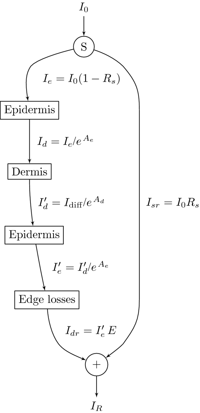

The parameters of the model are the specular reflection R _s, the absorption of the epidermis A _e, the absorption of the dermis A _d, and the edge loss coefficient E. From Eqs. 8, 9, it is apparent that the absorption in Eq. 10 is directly determined by the internal reflectance of because K, and the transport albedo [TeX:] $\mu^ {\prime} _{\rm a}$ ${\mu }_{\mathrm{a}}^{\prime }$ . The transport albedo, in turn, is a sum of all absorption and scattering properties of skin because [TeX:] $\mu _{\rm a} = \mu^ {\prime} _{\rm s} /(\mu^ {\prime} _{\rm s} + \mu _{\rm a})$ ${\mu }_{\mathrm{a}}={\mu }_{\mathrm{s}}^{\prime }/({\mu }_{\mathrm{s}}^{\prime }+{\mu }_{\mathrm{a}})$ . The absorption coefficient is a function of absolute chromophore concentrations, because [TeX:] $\mu^ {\prime} _{\rm a} = \sum\nolimits_{\it i} {\varepsilon _{\it i} (\lambda)c_{\it i} }$ ${\mu }_{\mathrm{a}}^{\prime }={\sum }_{\mathit{i}}{\varepsilon }_{\mathit{i}}\left(\lambda \right)c_{\mathit{i}}$ , where ɛ _i is the a priori known molar extinction coefficient of chromophore i. Therefore, the transport albedo can be calculated as follows:

Because [TeX:] $\mu^ {\prime} _{\rm a}$ ${\mu }_{\mathrm{a}}^{\prime }$ is a function of λ and c, so are T(λ, c), R _d(λ, c) and A _d(λ, c) as well. The BLL model of epidermis is A_e(λ,c_m) = ɛ_m(λ)c _m. The parameters for the edge-loss model, E(λ) are E _L and k. The total skin reflectance model can used in solving the concentrations, by adapting it to the measured reflectance spectrum, by minimizing the following square error over all spectral channels, i:

The E _SS can be minimized by finding optimal values for the parameters with LMA algorithm, for example. When the skin model is optimized, the derivative shown in Eq. 10 can be obtained.

The absorption difference between two locations of skin can now be written using Eqs. 6, 11 as a Taylor series,

The specular reflection is canceled when measuring the difference of two absorption spectra; therefore, it may be ignored. The possible edge loss needs to be compensated before applying Eq. 16. To keep the system linear, the higher order terms of the Taylor series cannot be used. The chromophore concentrations can be solved when the absorption coefficients, [TeX:] $\mu^ {\prime} _{\rm a}$ ${\mu }_{\mathrm{a}}^{\prime }$ , are replaced by concentrations and extinction coefficients,

Equation 17 contains four unknown concentrations. They can be solved by measuring the absorption change, ΔA, in at least at four different wavelengths, and finding an least-mean-squares (LMS) solution for each absorption. The wavelengths should be selected so that the equations are linearly independent. This can be arranged by selecting the wavelength sufficiently far away from each other. The absorption coefficients have unique spectra because they depend on the spectra of the extinction coefficients, ɛ.

2.4.

Reference Data Using Monte Carlo Simulation

To validate the proposed chromophore mapping technique, it was compared to the MCML simulation model. The MCML model consists of the model structure and the parameters. The structure is assumed to consists of homogeneous layers (shown in Fig. 4). The model was originally developed by Tuchin,³³ adopted by Reuss,¹⁵ and used, among others, by us.^{20, 22, 34}

Fig. 4

MCML skin-simulation model structure. The depths of the layers in millimeters are given along z-axis, in the left hand side. The layers of the skin model are shown in the right hand side. The incident and remitted light beams are shown in the top. The banana-shaped area is a schematic of the typical path for the photons contributing to the remittance shown by the arrow.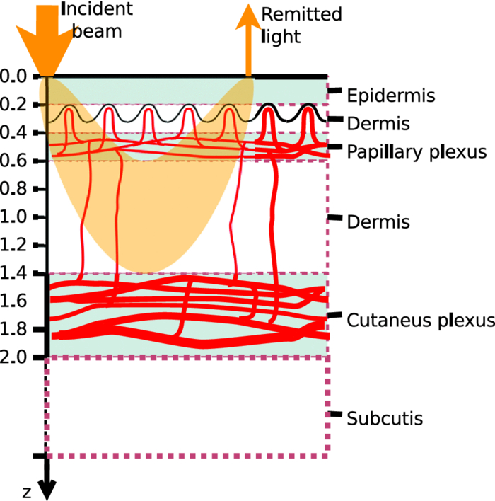

The parameters of each layer are the thickness, d, the absorption coefficient, μ _a, the scattering coefficient, μ_s, and the anisotropy, g. To be able to estimate the absorption coefficients, the skin chromophores and their concentrations are needed. In addition to hemoglobin and melanin, bilirubin and β-carotene may also affect to the concentration prediction. Water is only significant above 800 nm; it does not influence the skin color. The skin model was tuned to match palm skin over a range of different blood concentrations using the Allen's test, as described in Ref. 34. The nominal blood concentration is 150 g/l. The hemoglobin molar concentration in blood can therefore be calculated by dividing the concentration in grams/liter with the molar mass of hemoglobin; therefore,

The concentration of hemoglobin in skin is obtained by multiplying the hemoglobin concentration with the amount of blood in skin, the blood fraction, f _b. Therefore,

The typical value for f _b was 0.05 according to Reuss in Ref. 15. We have observed lower f _b values in our earlier studies, including, Ref. 34 where f _b ∈ [0.0016, 0.0045].

Often the absorption coefficient of melanin is modeled as follows:

The scattering of the tissue was modeled as a combination of Mie and Rayleigh scattering, as follows:³⁶

The skin without blood, the skin baseline, was simulated using following formula:³⁷

The variations in bilirubin concentration can potentially disturb the prediction of hemoglobin concentration or oxygen saturation. Therefore, the bilirubin concentration was varied in MCML simulation even though the prediction of the bilirubin content was not tried. The nominal bilirubin concentration in blood is C _Br = 10 μM/1. The bilirubin concentration was kept constant during “Blood” and “Melanin” data set simulation, and random values between the range, shown in Table 1 were selected in the simulation of the “Random” data set.

Fig. 8

Predictions of the chromophore concentrations of the Allen's test data set. Solid lines are predictions made by fitting the diffusion model to the full spectra. Dashed lines are obtained by fitting the diffusion model to selected five wavelengths, λ ∈ {505, 530, 595, 625, 850} nm. The predictions shown in the dotted lines are obtained by fitting the dMBLL model to the dif ference of the spectra. The reference spectrum is the one measured at time T = 4.4 s. (a) Fraction of oxyhemoglobin (o) in upper curve and the fraction of deoxyhemoglobin (Δ) in lower curve, (b) Predicted fraction of melanin (+) in skin, and (c) Predicted oxygen saturation levels.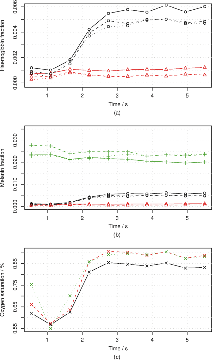

Table 1

Simulated data sets and the range of the parameters during the simulation.

The above skin model is used to generate four data sets, described in Table 1. The first two data sets are used for obtaining the numerical derivative of absorption by the melanin or blood concentrations for reference. The melanin set, contains 32 simulated skin spectra where all variables, except melanin concentration were kept constant. The melanin concentration was linearly distributed within a given range. In the blood data set, which also contains 32 simulated spectra, all variables except blood volume fraction, f _b, were kept constant. The blood fraction, f _b, was a linearly distributed within a given range. The random data set contains 104 simulated spectra, where independent random values were selected for melanin and blood concentrations from the given ranges.

Each simulated spectra, in each data set, contains 78 wavelengths in the range λ ∈ [380, 1050] nm. The simulations were made by tracking 10⁶ photons for each simulated wavelength. The plain MCML simulation estimates the reflectance of an infinite thin pencil beam.

2.5.

Allen's Test Data

In addition to the simulated data, the proposed algorithm was also validated using a measured data set. The measured data set consists of the reflectance spectra of the human skin from the palm of the hand from 20 persons, 5 locations each. From each location, a series of 10 consequent samples were measured at the rate of ∼1.8 samples per second. The measurements were carried out using an HR4000 spectrometer (Ocean Optics, Dunedin, Florida) and an ISP-REF integrating sphere (Ocean Optics). The measurement of the reflectance of the palm was acquired so that the test person placed his or her hand very lightly on the integrating sphere. The skin was illuminated with a diffuse light field over the whole aperture of the sphere, in which radius r _a = 0.5 cm, using a light source, built in the sphere. The reflectance was collected in the middle of the aperture, from the circular area, in which the radius is r _b = 0.15 cm. The experiment is further described in Ref. 34.

4.1.

Numerical Versus Analytical Derivatives

To validate the analytical derivatives shown in Eqs. 6, 11, they were compared to corresponding numerical derivatives obtained from the MCML data sets, melanin and blood, shown in Table 1. These data sets contain the absorption spectra when a single-chromophore concentration, either melanin or blood, is perturbed within a range, and all other parameters are kept unchanged. A third-order polynomial was fitted to the simulated A(c) curves, using statistical software package, R, and functional data analysis toolbox.³⁸ The derivatives of A(c) were now easily obtained by differentiating the corresponding polynomials. To study these polynomials and the first-order derivative over full reflectance spectra, the absorptions were differentiated by the concentrations instead of the absorption coefficients, and the procedure was repeated over the spectral range of λ ∈ [380, 1050] nm. The derivative of the absorption, A, by the absorption coefficient μ, and the derivative by the concentration are directly related because

The simulation results for Eq. 5 as a function of varying melanin concentrations are shown in Fig. 5a. The polynomial was fitted to the measured values of absorption as a function of melanin concentration, A(c _m), at each wavelength. Figure 5b displays the coefficients of the A(c _m) polynomial over all wavelengths.

Fig. 5

Absorption of skin by varying melanin fraction, f _m. (a) Absorption when the melanin fraction is increased from 1 to 4% in even steps of 0.095%. (b) Zeroth- (O), first- (Δ), and second- (+) order coefficients (not in scale) of the fitted polynomial A(c _m). The solid line shows the absorption when c _m = 0, and the dashed line shows the analytical derivative ∂A/∂μ_a,m.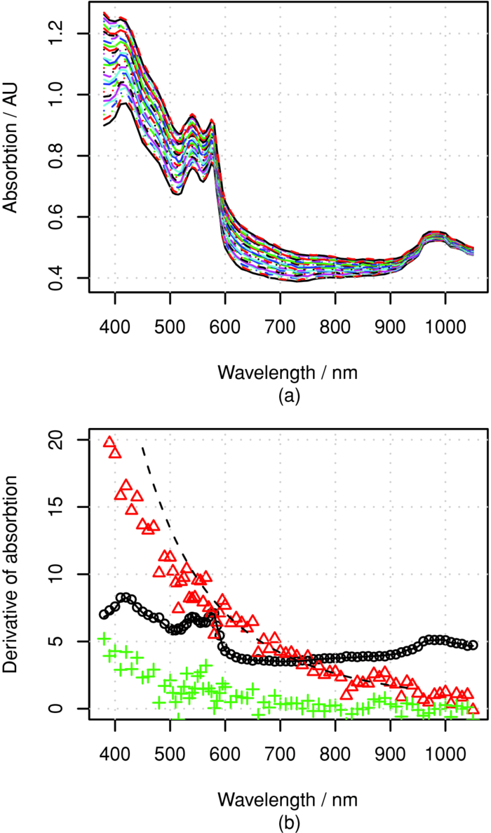

The zeroth-order coefficient of the polynomial and the skin absorption without melanin are, as expected, very close to each other. Correspondingly, the first-order coefficient and the analytical derivative are similar when the wavelength, λ > 550 nm. The numerical estimate if noisy, making the root-mean-square error-percentage (RMSEP) difference as large as 14%. For wavelengths at <550 nm, the behavior deviates from the Beer–Lambert law. The assumption of constant pathlength does not hold any longer because the absorption of melanin becomes very strong. The values of the second-order coefficient also seem to deviate from zero at wavelengths shorter than 550 or even 600 nm. The simple model shown in Eq. 6 seems work better at longer wavelengths.

4.2.

Absorption Versus Blood Concentration

The simulation results for Eq. 5 and the comparison to Eq. 11 are shown in Fig. 6. The constant term and the skin absorption without blood are significantly different at short wavelengths. This is because in addition to the linear term p _d, the derivative also contains the nonlinear blood effect, [TeX:] $\mu _{\rm a,b} p^{\prime} _{\rm d}$ ${\mu }_{\mathrm{a},\mathrm{b}}{p}_{\mathrm{d}}^{\prime }$ , and the cross-talk between skin baseline, [TeX:] $\mu _{\rm a,d} p^{\prime} _{\rm d}$ ${\mu }_{\mathrm{a},\mathrm{d}}{p}_{\mathrm{d}}^{\prime }$ . The numerical and analytical first-order derivatives are again similar (<550 nm). The explanation for larger differences in the range 450–500 nm is the absorption of bilirubin. Bilirubin was assumed to be solved in blood in MCML simulation but not in the diffusion model. Therefore, the derivative of MCML data contains also the absorption of bilirubin, but the diffusion model does not. This difference did not seem to significantly disturb the prediction of blood and melanin concentrations.

Fig. 6

Absorption of skin with varying blood concentration. (a) Absorption when the skin blood fraction is increased from 0 to 1% in even steps of 0.031%. (b) Zeroth- (O) and first-(Δ) order coefficients of the fitted polynomial A(c _m) (zeroth-order polyno mials is multiplied by 30), the coefficients of the absorption polynomial, A, by blood concentration c _b. The solid line shows the corresponding analytical derivative.

4.3.

Comparison to Monte Carlo Simulation

The accuracy of the prediction of the chromophore concentrations is assessed by means of the random MCML simulation data set, shown in Table 1. The results are displayed in Fig. 7. The accuracy of the prediction is measured as the RMSEP error and Pearson correlation coefficient between the predicted and given values. The prediction of the melanin content is the most accurate. Blood-prediction performance is slightly weaker than prediction for melanin because the relationship between the blood concentration and absorption is curved. The prediction of oxygen saturation is the weakest. Often the concentration of deoxyhemoglobin is very low, and even small absolute errors cause large relative errors. Sometimes even slightly negative values were observed. If negative concentration was observed, then it was saturated to zero. The samples shown as triangles are these kinds of fixed predictions.

Fig. 7

Prediction of the chromophore concentrations of the MCML simulation using dMBLL and following wavelengths: λ ∈ {505, 530, 595, 625, 850} nm. (a) Predicted blood fraction against blood fraction used in the MCML simulation. The prediction error is RMSEP=15% and the correlation between predicted and given values, r=0.94. (b) Predicted fraction of melanin against the melanin fraction used in MCML simulation. The prediction error RMSEP=7% and correlation r=0.99. (c) Predicted oxygen-saturation levels against saturation levels in the MCML simulation. RMSEP=10%, r=0.73.

4.4.

Allen's Test Data

The algorithm was applied to the experimental Allen's test data to study its performance for measured data. The results are shown in Fig. 8. The prediction of each chromophore was done with three different methods. First by fitting the skin model to the spectra by optimizing the chromophore concentrations with LMA (solid line). Then the same method was repeated, but now only five selected wavelengths were used (dashed lines). The third method is to use the analytical derivative and Eq. 17 to solve the linearized skin model around and operating point. The spectrum measured at time T = 4.4 s was used as an operating point.

4.5.

Execution Speed

To evaluate the speed benefit gained by using a closed-form dMBLL solution, the predictions done above were benchmarked. The diffusion model and the dMBLL implementations were programmed with a statistical software package, called R. The MCML program was programmed with C. The predictions were run in a normal desktop PC. The processor of the PC was Intel^®Core 2 CPU 6600 using a 2.40-GHz clock frequency. We also estimated how long it would take to process every pixel in a 1-megapixel image. The results of the benchmarks are shown in Table 2.

Table 2

The Speeds of different implementations.