|
|
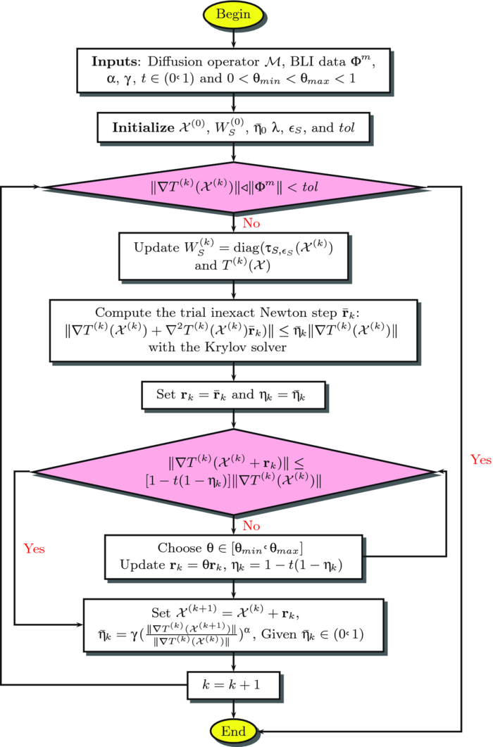
1.IntroductionFrom being the solid development of bioluminescent probes and reporter technologies,1, 2, 3 the application of bioluminescence in biomedical in vivo imaging has become more and more attractive over the recent years. It offers an alternative opportunity for noninvasively visualizing biological processes at the physiological and molecular levels in whole animals.4, 5, 6 Tomographic bioluminescence imaging (TBI) can further translate the planar imaging information into three-dimensional bioluminescent source distribution quantitatively, thus greatly facilitating applications in related biomedical in vivo studies.7, 8 Therefore, the development of the reconstruction approaches for tomographic imaging plays a unique role in the achievement of practical biomedical in vivo imaging studies. Nevertheless, it is known that the inverse problem of tomographic imaging is an ill-posed problem due to the fact that some limited information can only be measured from the boundary of animals to estimate the internal bioluminescent source distribution.9 Therefore, this imaging modality faces various challenges in its accuracy and reliability. Researchers have made considerable efforts to cope with the ill-posedness of the underdetermined inverse problem. It can be alleviated by incorporating some a priori information. Spectrally resolved boundary measurements, which practically increase the amount of independent data, are necessary to accurately recover tomographic images of bioluminescent sources.10, 11, 12, 13, 14 By reducing the number of unknowns, the permissible source region method is demonstrated to be capable of correctly reconstructing the images at monochromatic measurements.15, 16, 17 This reconstruction domain is needed to be spatially constrained to the area of interest, whereas, it is not always feasible to define such a region effectively in practical tomographic imaging applications. Moreover, the varying boundary conditions have also been proposed to enhance the reliability of the reconstruction results.18 On the other hand, the regularization strategies, which are imposed with the output-least-squares formulation to stabilize the inverse problem, are also indispensable for tomographic quality.19 Although the l 2-type regularization strategy is the most popular and commonly-applied, it often imposes over-smoothing on the reconstruction results. In contrast, due to the high specificity of the bioluminescence probes and reporter technologies, the objective for tomographic imaging is only the sparsely-distributed signal. Consequently, the sparse prior knowledge can be employed to recover the source distribution and preserve discontinuities in the reconstructed profiles with less measurements, which is presented in references by Lu 20 and Gao and Zhao.21 Actually, the sparse-type (l 1) regularization has been studied for years and recently has drawn a lot of attention due to theoretical justification and many applications. 20, 22, 23, 24, 25, 26, 27 Although the aforementioned methods have been proposed to overcome the challenges in the inverse problem, further study is still needed to alleviate the dependence with some parameters during reconstructions, such as the parameters in the regularization term. In general, it is assumed that there are multiple local minima of the objective function in the TBI inverse problem.28 Consequently, the application of local optimization techniques, e.g., the conventional Newton-based optimization methods that explore the unknown parameter space only near a single local minimum, may lead to inapposite convergence without finding the global minimum.16, 17, 29, 30 As a consequence, reconstructions on a part of the animal body or even on the whole body become more difficult. Recently, a graph cuts-based method was proposed, which could find a global optimal solution efficiently and was not dependent on a starting unknown guess in the search process.31 However, since the reconstruction could only be represented in discrete form, it was difficult to recover complex source distribution appropriately in whole animals. Likewise, more efforts are urgently needed to make whole body imaging available with an arbitrary initial guess for the unknowns. In this work, a dynamically-sparse regularized global method is proposed. In order to make full use of the sparse a priori information, the sparse term l p (1 ⩽ p < 2) is approximated by a corresponding weighted l 2 norm in each iteration,32 rather than be adopted directly. It can facilitate the generalization of the sparse regularization with greater flexibility of p in the dynamic quadratic frame, and avoid tedious numerical operation as well. A globally-converged optimization technique is presented to search for the global solution. It could find the globally optimal solutions far from the starting unknown guess efficiently, and maintain the reliable reconstruction quality over a wide-range of regularization parameters. In Sec. 2, we present the proposed method for TBI. In Sec. 3, validations based on an in vivo experimental data set demonstrate higher imaging reliability and cheaper computational cost of the proposed method. First reconstruction comparisons of the proposed method with other methods demonstrate the applicability on the entire region. Then, the reliable performance on various ranges of regularization parameters and initial unknown values is also validated. Based on the in vivo mouse experiment and a mouse atlas, the tolerance for optical property mismatch is investigated with optical overestimation and underestimation on absorbing and reduced scattering properties. Additionally, the reconstruction efficiency is also analyzed with different sizes of mouse grids. Finally, we discuss and conclude this paper. 2.Methods2.1.Forward ModelIn the steady-state domain, the forward problem of light propagation for TBI can be modeled as a diffusion approximation to the radiative transport equation,16 which is given by Eq. 1[TeX:] \documentclass[12pt]{minimal}\begin{document} \begin{equation} -\nabla \cdot (D(\textbf {r})\nabla [\Phi (\textbf {r})]+ \mu _{a}(\textbf {r})\Phi (\textbf {r})=\mathcal {X}(\textbf {r}) (\textbf {r}\in \Omega). \end{equation} \end{document}In the bioluminescence imaging experiments, the whole process is performed in a completely dark environment, and there is no external photon into imaging domain Ω through its boundary ∂Ω, so the Robin-type boundary condition is suitable: Eq. 2[TeX:] \documentclass[12pt]{minimal}\begin{document} \begin{equation} \Phi (\textbf {r})+2\kappa (\textbf {r},n,n^{\prime })D(\textbf {r}) [\textbf {v}(\textbf {r})\cdot \nabla \Phi (\textbf {r})] =0 (\textbf {r}\in \partial \Omega). \end{equation} \end{document}Eq. 3[TeX:] \documentclass[12pt]{minimal}\begin{document} \begin{equation} V(\textbf {r})=-D(\textbf {r}) [\textbf {v}(\textbf {r})\cdot \nabla \Phi (\textbf {r})] =\frac{\Phi (\textbf {r})}{2\kappa (\textbf {r},n,n^{\prime })} (\textbf {r}\in \partial \Omega). \end{equation} \end{document}Based on the finite element theory, Eqs. 1, 2 are discretized by piecewise linear finite elements, and a matrix-vector equation is integrally assembled.33 Consequently, after a series of rearrangements for the elements in the matrix, the linear relationship between the measured photon density distribution and the unknown source distribution in heterogeneous biological tissues is established as: Eq. 4[TeX:] \documentclass[12pt]{minimal}\begin{document} \begin{equation} \mathcal {MX}=\Phi, \end{equation} \end{document}2.2.Dynamic Sparse Regularized FunctionIn practice, the common approach for the TBI inverse problem is to adopt the output-least-squares formulation. A regularization function is incorporated to stabilize the inversion problem like this: Eq. 5[TeX:] \documentclass[12pt]{minimal}\begin{document} \begin{equation} S(\mathcal {X})=||\mathcal {LX}||_{p}^{p}, \end{equation} \end{document}Eq. 6[TeX:] \documentclass[12pt]{minimal}\begin{document} \begin{equation} T(\mathcal {X})=\frac{1}{2}\Vert \mathcal {MX}-\Phi ^{m}\Vert _{2}^{2}+\lambda ||\mathcal {LX}||_{p}^{p}, \end{equation} \end{document}Eq. 7[TeX:] \documentclass[12pt]{minimal}\begin{document} \begin{equation} S(\mathcal {X})=\frac{1}{p}\Vert \mathcal {X}\Vert _{p}^{p} (1\le p< 2). \end{equation} \end{document}Now let us begin to construct the dynamic sparse regularized function. Instead of solving the sparse l p problem,20 a quadratic version is generated to approximate the sparse term for each iteration.32 In order to replace the l p term by the l 2 one and dynamically regularize the objective function, the quadratic function is defined as: Eq. 8[TeX:] \documentclass[12pt]{minimal}\begin{document} \begin{equation} Q_{S}^{(k)}(\mathcal {X})=\frac{1}{2}\big \Vert W_{S}^{(k)^{1/2}}\mathcal {X}\big \Vert _{2}^{2} +\left (1-\frac{p}{2}\right)S(\mathcal {X}^{(k)}), \end{equation} \end{document}Eq. 9[TeX:] \documentclass[12pt]{minimal}\begin{document} \begin{equation} W_{S}^{(k)}=\hbox{diag} [\tau _{S,\epsilon _{S}}(\mathcal {X}^{(k)})]. \end{equation} \end{document}The diagonal matrix [TeX:] $W_{S}^{(k)}$ is updated in each iteration using the values of the last step. The matrix actually plays a spatially varying role to maintain the imaging results reliable enough, which can tolerate different orders of magnitude of regularization parameters to obtain reliable results to some extent. Based on the strategy in the reference by Rao and Kreutz-Delgato,37 [TeX:] $\tau _{S,\epsilon _{S}}$ (for some small εS) is defined as Eq. 10[TeX:] \documentclass[12pt]{minimal}\begin{document} \begin{equation} \tau _{S,\epsilon _{S}}(u) = \left\lbrace \begin{array}{@{}l@{\quad}l} \mid u\mid ^{p-2} & \hbox{if\quad $\mid u \mid >\epsilon _{S}$} \\[3pt] 0 & \hbox{if\quad $\mid u \mid \le \epsilon _{S}$} \end{array}. \right. \end{equation} \end{document}Note that it is necessary to add the constant term [TeX:] $(1-\frac{p}{2})S(\mathcal {X}^{(k)})$ in Eq. 8 to ensure that: Eq. 11[TeX:] \documentclass[12pt]{minimal}\begin{document} \begin{equation} S(\mathcal {X}^{(k)})=Q_{S}^{(k)}(\mathcal {X}^{(k)}) (\hbox{as} \epsilon _{S}\rightarrow 0), \end{equation} \end{document}Eq. 12[TeX:] \documentclass[12pt]{minimal}\begin{document} \begin{equation} S(\mathcal {X})<Q_{S}^{(k)}(\mathcal {X}) (\forall \mathcal {X}\ne \mathcal {X}^{(k)}), \end{equation} \end{document}Eq. 13[TeX:] \documentclass[12pt]{minimal}\begin{document} \begin{equation} \nabla _{\mathcal {X}} S(\mathcal {X})\mid _{\mathcal {X}=\mathcal {X}^{(k)}}=\nabla _{\mathcal {X}} Q_{S}^{(k)}(\mathcal {X})\mid _{\mathcal {X}=\mathcal {X}^{(k)}}\!\!. \end{equation} \end{document}It is noteworthy that the original regularization term [Eq. 7] and its quadratic version [Eq. 8] have the same value and tangent direction at [TeX:] $\mathcal {X}=\mathcal {X}^{(k)}$ . Thus, based on the dynamic sparse regularization technique, the objective function is reformulated into the following quadratic form: Eq. 14[TeX:] \documentclass[12pt]{minimal}\begin{document} \begin{eqnarray} T^{(k)}(\mathcal {X})&=&\frac{1}{2}\Vert \mathcal {MX}-\Phi ^{m}\Vert _{2}^{2}+\lambda Q_{S}^{(k)}(\mathcal {X})\nonumber \\ &=&\frac{1}{2}\Vert \mathcal {MX}-\Phi ^{m}\Vert _{2}^{2}+\frac{\lambda }{2}\big \Vert W_{S}^{(k)^{1/2}}\mathcal {X}\big \Vert _{2}^{2}\nonumber \\ &+&\lambda \left(1-\frac{p}{2}\right)S(\mathcal {X}^{(k)}) (k\ge 0). \end{eqnarray} \end{document}The corresponding gradient and Hessian matrix are easily derived 15.In particular, if p = 2 and εS = 0, [TeX:] $Q_{S}^{(k)}(\mathcal {X})=\frac{1}{2}\Vert \mathcal {X} \Vert _{2}^{2}$ for any k, thus the dynamically sparse regularized function degrades into the popular static regularized quadratic objective function.16, 20, 31 2.3.Reconstruction AlgorithmAfter constructing the dynamically sparse regularized function for the inverse problem, the reconstructed solution can be estimated by minimizing the objective function dynamically: Eq. 16[TeX:] \documentclass[12pt]{minimal}\begin{document} \begin{equation} \mathcal {X}_{recons.}=\arg \mathop {\min _{\mathcal {X}}}T^{(k)}(\mathcal {X}), \end{equation} \end{document}Eq. 17[TeX:] \documentclass[12pt]{minimal}\begin{document} \begin{equation} \nabla T^{(k)}(\mathcal {X})=0. \end{equation} \end{document}One kind of widely applied algorithm for solving Eq. 17 is the Newton method, as shown in Algorithm: where [TeX:] $\textbf {r}_{k}$ denotes the increment step at kth iteration. This method exactly solves Newton's equations (step 3 in Algorithm) at each iteration, which can be very expensive if the number of unknowns is large and may not be justified when [TeX:] $\textbf {r}_{k}$ is far from a solution. Thus, an inexact Newton method is preferred to just compute an approximate solution of Newton's equations at each iteration, which can be summarized in pseudo-code as follows:38 Table 1Newton method.
Such approximate treatmental offers a trade-off between the accuracy with a solution of Newton's equations and the amount of the computational cost per iteration. By making the ηk appropriately small, the convergence can be made and the norm of [TeX:] $\nabla ^{2} T^{(k)}(\mathcal {X})$ can be reduced.39 Since [TeX:] $\nabla ^{2} T^{(k)}(\mathcal {X}^{(k)})\textbf {r}_{k}\break +\nabla T^{(k)}(\mathcal {X}^{(k)})$ is the residual of Newton's equations, each ηk denotes how accurate [TeX:] $\textbf {r}_{k}$ is close to the exact solution. It is seen that [TeX:] $\textbf {r}_{k}$ satisfying step 4 in Algorithm is an inexact Newton step. Table 2Inexact Newton method.
If the inexact Newton condition (step 4 in Algorithm) is augmented with a sufficiently decreased condition for [TeX:] $\nabla T^{(k)}(\mathcal {X})$ , the algorithm above can be globally converged:38 Eq. 18[TeX:] \documentclass[12pt]{minimal}\begin{document} \begin{eqnarray} \Vert \nabla ^{2} T^{(k)}(\mathcal {X}^{(k)}\!+\textbf {r}_{k})\Vert \le [1\!-\!t(1-\eta _{k})]\Vert \nabla T^{(k)}(\mathcal {X}^{(k)}\Vert, t\in (0,1).\nonumber\!\!\!\! \\ \end{eqnarray} \end{document}However, a backtracking strategy is alternatively adopted to transform the augmented condition [Eq. 18] into a practical formulation. At each iteration, an initial inexact Newton step at a specified level is tried, and if it proves unsatisfactory, the inexact Newton steps to higher levels that are solved until a reliable enough step is obtained. The detailed backtracking strategy is shown as: Table 3
Hence, the inexact Newton method with backtracking strategy is incorporated together to enhance convergence from an arbitrary initial guess for unknowns. Up until the end, the proposed reconstruction method is established for the TBI inverse problem. The algorithm shown in Fig. 1 summarizes how the global inexact Newton approach takes advantage of a dynamically sparse regularization technique. The flowchart includes dual-level iterations. The outer iteration controls the whole inexact algorithm, and the sparse regularization term is updated based on the previous iteration during each outer iteration. In order to maintain accuracy of the approximation for [TeX:] $Q_{S}^{(k)}(\mathcal {X}^{(k)})=S(\mathcal {X}^{(k)})$ , the small εS is set as 0.02. The inner iterations also fall into two parts: the Krylov solver and the backtracking operation. Here, the preconditioned conjugate gradient is selected as the Krylov solver. p = 1 is taken as an example in Eq. 14. 3.ResultsIn this section, an in vivo heterogeneous mouse reconstruction experiment was implemented to demonstrate the feasibility of the proposed method. The experiment was performed on the dual-modality optical/micro-CT in vivo imaging system developed by our group.31, 40, 41 The optical detector was a highly sensitive CCD camera (VersArray, Princeton Instruments, Trenton, New Jersey) coupled with a lens (Nikkor, Nikon, Japan). The bioluminescent source was simulated by a home-made luminescent bead, which had an emission spectrum similar to that of a firefly luciferase-based source. Its dimension was about 1.5 mm in diameter and 2.5-mm long. A nude hairless mouse (Nu/Nu, Laboratory Animal Center, Peking University, China) was adopted in this experiment. Before optical and x ray data acquisition, the CCD was refrigerated to −110°C to reduce dark current noise, and the mouse was anesthetized and the bead was implanted stereotactically into the interspaces between the left and right lobes of the liver. The optical data was collected first. Bioluminescence images from four views were acquired from the mouse surface, with 60 s integration time for each image, and then four corresponding white mouse images were also obtained. After finishing optical acquisition, the mouse was scanned using the micro-computed tomography (CT) to obtain the surface and anatomical structure. Data processing followed data acquisition. The mouse structure images were reconstructed by the CT cone-beam reconstruction algorithm.42 Then, the data were segmented into a heterogeneous volumetric mesh for image reconstruction, as shown in Fig. 2c. This mesh contains 23,752 tetrahedral elements and 4560 discretized nodes with 1092 nodes on the surface. The torso applied for reconstruction covered over 60% of the volume of the mouse body. Then, the demanded photon density projections on the mouse surface were obtained, and the main procedure is summarized in Fig. 2. First, the two sets of data were spatially registered by the corresponding markers on 2D optical images and on 3D CT volume, which is shown in Fig. 2. The image registration results in Fig. 2d were obtained by incorporating Figs. 2a and 2b. Second, the complete-angle outgoing photon density on the mouse surface [Fig. 2f] was projected from the 2D images on the CCD [Fig. 2e] to the 3D surface [Fig. 2c] according to the co-registered image [Fig. 2d]. The source was easily distinguished in CT images, and the actual position of the source could be confirmed at (25.54, 21.31, 8.52), as shown in Fig. 2a. Additionally, the optical properties for each organ were determined with the inverse adding doubling scheme,43 as listed in Table 1. Fig. 2The dual-modality fused image co-registration and the corresponding outgoing optical density projection on the mouse surface. (a) The original CT volume obtained by the micro-CT component of the dual-modality system. (b) The white images of the mouse from four views. (c) The heterogeneous grid of a mouse torso CT image, including heart, lungs, liver, muscle, and bone. (d) The fusion registration by markers between the CT image in (a) and the white mouse images in (b). (e) The measured bioluminescence images from four views captured by the optical component. (f) The final 360°-projected outgoing photon density on the mouse surface. It is the fusion result of (c), (d) and (e).  Fig. 11The reconstruction time comparisons of imaging reconstruction on four different grids. Note that the time is scaled using 10 logarithmic forms in the axis of ordinate. 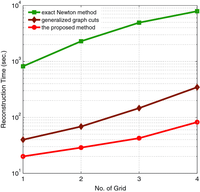 Table 1Optical properties for each organ in the mouse.
3.1.Reconstruction ComparisonBased on the in vivo mouse experiment, the proposed method was first evaluated by comparing it with other methods. One of the exact Newton methods (as in Algorithm) was selected to demonstrate the predominance of the global inexact Newton method. A recently developed gradient-free method, which was generalized graph cuts, was also employed to further demonstrate the potential and effectiveness of the proposed method.31 This method also has the property of global convergence.44 As reported previously,16, 17, 30, 31 the reconstruction on a large region often results in troublesome problems when using the exact Newton-type method, and a permissible source region is preferred to reduce the number of unknowns and keep reliable reconstruction results. Figure 3 shows the comparison of the reconstruction results for these methods. The cross sectional images based on the exact Newton method are shown in Figs. 3c and 3(d). The permissable source region in Fig. 3c is {(x, y, z)|22 ⩽ x ⩽ 28, 17 ⩽ y ⩽ 23, 6 ⩽ z ⩽ 10}, and the result in Fig. 3d is reconstructed on the whole region as depicted in Fig. 2c. It is obvious that the selection of the permissable source region is very necessary to obtain reliable reconstruction results. If the permissable region is extended or even no permissable region is adopted, and more unknowns are introduced in the reconstruction, the reconstructed source distribution may deviate further from the real one further, as shown in Fig. 3d. In contrast to this method, as shown in Fig. 3e, both accurate source localization and distribution can be recovered based on the global inexact Newton method applied on the entire region. The reconstruction image in Fig. 3b is the result based on generalized graph cuts. Both of the proposed and generalized graph cuts methods can localize source distribution well compared with the true one. However, the proposed method can also quantify source density, but this was not the case of the gradient-free method. In the reconstructions based on the Newton method and generalized graph cuts, the best regularization parameters were selected and the parameters were in the range of 10−5 to 10−3. For the proposed method, the value was 4 × 10⁻². Fig. 3The comparison of cross sectional images for reconstructed bioluminescence source distribution. (b) The result of generalized graph cuts method on the whole reconstruction region. (c) and (d) The result of the Newton method on a small permissable source region and the whole reconstruction region, respectively. (e) The result of the proposed method on the entire reconstruction region. (a) and (f) are the corresponding CT slices. Note that the colorbar scales on the right vary with each reconstruction. 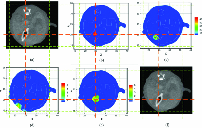 3.2.Reliability Studies for Imaging ReconstructionsIn this part, reconstructions regularized with different orders of magnitude (10−1 to 10−12) parameters were performed for in vivo tomographic bioluminescence imaging. As shown in Fig. 4, reconstructions were hardly affected with the regularization parameters, and the bioluminescent source distribution was accurately reconstructed in all cases. Moreover, the results also offered little difference in the way of quantitative information. Figure 5 further demonstrates the nonsensitive performance of the proposed method with a large range of regularization parameters. During four outer iteration steps, the evolution curve of [TeX:] $||\mathcal {MX}-\Phi ^{m}||/||\mathcal {M}^{t}\Phi ^{m}||$ was almost the same with each other, thus only one curve was given here. It appears that the regularization parameters may not affect the tomographic imaging quality very much. Fig. 4Reconstruction results with different regularization parameters. The center is the corresponding CT slice. All of the unknowns are set to be 0 for all cases.  Fig. 5The evolution curve of [TeX:] $||\mathcal {MX}-\Phi ^{m}||/||\mathcal {M}^{T}\Phi ^{m}||$ as a function of the iteration steps with initial unknowns of 0 uniformly. Four outer iteration steps are undergone during reconstruction. Note that the curve with different regulation parameters is very similar, hence just one curve is plotted here.  Second the reliability of the proposed method was further validated by changing the initial guess for unknowns [TeX:] $\mathcal {X}^{(0)}$ , which were uniformly distributed in a range from 0 to 200. In Fig. 6, based on the results shown above, the bioluminescent source distribution was recovered credibly, and the reconstructions were hardly affected with initials in all cases. Moreover, the results also represented similarly quantitative information with each other. Similar to the curve in Fig. 5, it is also further demonstrated in Fig. 7 that the proposed method can tolerate different initial unknowns and converge reliably. It is also interesting that during iteration, the evolution values of [TeX:] $||\mathcal {MX}-\Phi ^{m}||/||\mathcal {M}^{t}\Phi ^{m}||$ for large initial values would merge into one curve sooner or later, which is almost the same with each other. It is demonstrated that, as proven mathematically,38 the global inexact Newton method with dynamic sparse regularization is globally optimized, and the tomographic imaging quality can be maintained. Fig. 6Reconstruction results with different initial guesses. The initials are uniform for all unknowns. The center is the corresponding CT slice. The regularization parameter in all cases is selected as 4 × 10⁻².  Fig. 7The evolution curve as a function of iteration steps with different initial unknowns. Four outer iteration steps are undergone.  Moreover, it is noteworthy that all reconstructions were performed on the whole grid, instead of being performed on small permissible source regions. In the mouse experiments, it is not always reliable or feasible to define such regions effectively, so the proposed method is highly applicable to practical tomographic imaging. 3.3.Evaluation of the Tolerance for Optical Property MismatchBased on the advantage of heterogeneous tissue distribution, the optical property in each organ makes an indispensable role for high quality imaging reconstruction. When constructing heterogeneous optical property distribution, a simple and convenient option is to introduce average parameter values from measured or published ranges for individual data.30, 45, 46, 47 Although this approach may not be as accurate as straightforward parameter measurements on individual animals, its limitation could be a trade-off for its simplicity and avoidance of additional operations. Here, the reconstruction performance that results from the mismatch in optical properties was evaluated. Two mouse models were employed here, including the above-mentioned experimental mouse and a mouse atlas (which contains 25,783 tetrahedral elements and 4614 nodes with 486 nodes on the surface), as shown in Fig. 8. The atlas was also constructed by our group, and the optical properties for each tissue are listed in Table 1. More details about the atlas can be found in Liu et al.31 Based on the mouse atlas, the case with the two sources were considered for evaluating the tolerance for optical property mismatch. For the two models, the optical property mismatch of ±20% and ±50% in both μa and [TeX:] $\mu ^{\prime }_{s}$ was introduced into the tissues. Practically, the optical properties may have a combination of positive and negative mismatch of different magnitudes in the absorption and scattering properties. Consequently, four extreme conditions for all of the tissues were considered here: both μa and [TeX:] $\mu ^{\prime }_{s}$ were overestimated; both μa and [TeX:] $\mu ^{\prime }_{s}$ were underestimated; μa was overestimated, [TeX:] $\mu ^{\prime }_{s}$ was underestimated; μa was underestimated, and [TeX:] $\mu ^{\prime }_{s}$ was overestimated, as listed in Table 2. Fig. 8The volumetric mesh of the heterogeneous mouse atlas, including heart, lungs, liver, spleen, muscle, and bone.  Table 2The summary for the effect of optical property mismatch of ±20% and ±50% in both μa and $\mu ^{\prime }_{s}$ μs′ . OP. mismatch denotes the bias from real optical properties.
The Monte Carlo (MC) method is accurate for the simulation of photon propagation through biological tissues. In the mouse atlas experiment, a MC-based molecular optical simulation environment was employed here to statistically estimate the bioluminescence signal distribution on the mouse surface.48, 49 In the simulation settings, two spherical solid sources with a radius of 1.0 mm were located at (22.00, 34.00, 10.00) and (21.50, 34.00, 15.00). A total of 106 photons for each source were tracked for enhancing simulation accuracy. The reconstruction results are summarized in Table 2, and typical results are shown in Fig. 9. In general, both the mouse and the mouse atlas, the bioluminescent sources were reliably reconstructed. The reconstruction offset is summarized in Fig. 10. In the first case, the maximum location error was 2 mm when there was a –50% mismatch for both μa and [TeX:] $\mu ^{\prime }_{s}$ (No. 6 of model 1); in the second case, the maximal error occurred when a +50% mismatch both in μa and [TeX:] $\mu ^{\prime }_{s}$ (the second source in No. 5 of model 2) existed with ∼2 mm offset as well. From Table 2, it is observed that the reconstructed sources were localized less ideally with ±50% errors than with ±20%. It consequently seemed that the effects of the mismatch on the tomography results became larger for increasing optical errors. With the mismatch increasing, an artefact also appeared around the source regions [as the red arrow in Fig. 9b], which may be an inevitable side-effect for large optical property errors.50 Fig. 9The reconstruction results for both models when an optical property mismatch is introduced. (a) and (b) are results based on the experimental mouse, and (c) and (d) are based on the mouse atlas. (a) and (c) The results with +20% mismatch of both μa and [TeX:] $\mu ^{\prime }_{s}$ . (b) and (d) The results with mismatch of +50% μa and −50% [TeX:] $\mu ^{\prime }_{s}$ . In (b), the red arrow points to the artifact around the real source. 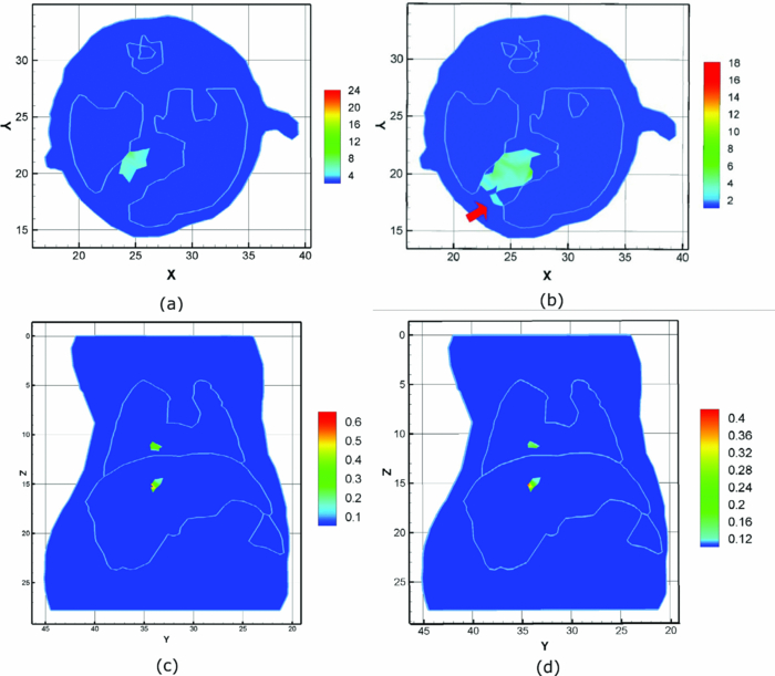 Fig. 10Comparison for the source localization offset with different optical property mismatch. (a) The localization offset of the experimental mouse. (b) The localization offset for two sources based on the mouse atlas.  Another interesting effect seemed that errors in opposite directions partially cancelled each other out, leading to improved source localization. As plotted in Fig. 10, when all tissues had +50% errors in μa and −50% errors in [TeX:] $\mu ^{\prime }_{s}$ or −50% errors in μa and +50% errors in [TeX:] $\mu ^{\prime }_{s}$ [No. 5, 6 in Figs. 10a and 10b], the localization errors were much better than those with the same sign, and were similar to those with ±20%. The artifacts also appeared to affect the imaging quality only in the same direction with a 50% error (−50% errors for model 1, and ±50% for model 2). Moreover, the reconstructed source became more diffuse with greater errors, compared with lower optical errors. A typical comparison is shown in Figs. 9a and 9b. In other words, when optical errors with the same sign occurred during reconstruction, the imaging quality would be degraded further. The imaging quality based on the mouse atlas was better than that of mouse experiment. The results in Fig. 9c for +50% errors in μa and -50% errors in [TeX:] $\mu ^{\prime }_{s}$ were very similar to that of the +20% errors in μa and −20% errors in [TeX:] $\mu ^{\prime }_{s}$ in Fig. 9d. The major reason may be the inevitable discrepancies in the optical properties for the experimental mouse tissues. In practice, it is impossible to obtain accurate optical values.47, 50 The source in the experimental mouse was located between the left and right lobes of the liver, thus the space was relatively narrow, and the diffuse approximation-based forward model may not fully deal with this special case, which is another affecting factor. Higher order approximation-based models may be helpful for higher imaging quality in narrow structures.51, 52 For all of the reconstructions based on the two mouse models in this part, the regularization parameter was set as 4 × 10⁻², and the unknowns were uniformly initialized as zero. It is worth addressing that, based on the mouse atlas using other values of the regularization parameter and the initial unknown guess, the tomography results can be obtained with similar imaging quality as shown in Table 2. 3.4.Efficiency Studies for Imaging ReconstructionsThe high efficiency of the proposed method was also investigated, compared with the exact Newton method, and the generalized graph cuts (GGC) method. As listed in Table 3, four discrete grids of varying sizes of the experimental mouse were utilized. Table 3Efficiency comparisons of imaging reconstructions. The size of the grid means the number of points × the number of elements.
Based on the different methods, the reconstruction time of the four grids is also summarized in Table 3. The reconstruction cost of the global inexact Newton method was much cheaper than the exact Newton one. The efficiency of the proposed method was about 1 to 2 orders-of-magnitude of the exact method. As the grid dimension increased, efficiency predominance became larger, which is also shown in Fig. 11. The key factor is that in the proposed method, only the approximate rather than the exact solution was computed for the next iteration. Moreover, while the efficiency of GGC was also much higher than the exact Newton method, the performance of the proposed method overcame the GGC, which is also clearly depicted in Fig. 11. The reason lay in the complex process for the pairwise terms in the unstructured grid (not based on square pixels or tube vortexes).31 On the unstructured grid, the neighborhood for each node was uncertain, and there were more neighbor nodes around a node than the structured grid (based on square pixels or tube vortexes). This process involved a time-consuming operation. Hence, it is seen that the proposed method was very efficient, and was also promising for the inverse problem of TBI. All of the simulations were done on a Intel Core 2 Duo 1.86 GHz PC with 3 GB RAM. 4.Discussions and ConclusionIn this study, we proposed an efficient global inexact Newton method with a dynamic sparse regularizer for in vivo TBI. In order to make full use of a priori information of the source sparse-distribution, the sparse regularizer is dynamically approximated by a corresponding weighted quadratic norm in each iteration, rather than being adopted explicitly. The inexact Newton with a backtracking optimization technique has the capability to search for the global optimal solution among multiple local minima of the objective function. The in vivo mouse experiment shows that the proposed method can significantly enhance the reconstruction robustness of the regularization parameter and initial values with no a priori assumptions on the bioluminescent source biodistribution. Applying both the experimental data and the Monte Carlo-based mouse atlas data, the sensitivity evaluation for optical property mismatch indicates that even when there exist up to 50% overestimate and underestimate errors in the heterogeneous mouse models, this method can still maintain adequate reconstruction quality. During the reconstructions, it exhibits high computational efficiency and reliable convergence behavior in TBI reconstructions. To summarize, it is demonstrated that the proposed method bears a strong potential to improve the reconstruction capacity for practical tomographic imaging applications. Generally, data fusion from different modalities plays an indispensable role for high imaging fidelity,53, 54, 55 as specially in tomographic bioluminescence imaging, and it is also necessary to combine the information from optical and micro-CT modalities. The data fusion between bioluminescence imaging and micro-CT is helpful to alleviate the ill-posedness and improve imaging quality. First optical images and CT volume can be spatially co-registered, and the captured 2D bioluminescent signal can be projected onto the 3D mouse surface. Second the heterogeneous anatomical structure by micro-CT is naturally fused through the construction of the optical forward model. The fusion imposes such useful a priori information that accurate reconstruction results can be estimated. Moreover, although the anatomical map has been incorporated in the forward model, the heterogeneous priors can also be employed in the inversion process.36 Furthermore, although the diffusion approximation model for TBI reconstructions is very popular, more accurate forward models to describe photon propagation in biological tissues are also necessary for higher imaging quality. Since the emission spectra peaks of the four main luciferase enzymes (Fluc, BGr68, CBRed, and hRluc) are 612, 543, 615, and 480 nm at temperature 37 ○C, respectively, a significant part of the emission spectra deviates from the high-scattering and low-absorbing window. Moreover, when light propagates through a geometrically small volume, the diffusion assumption also becomes invalid to some extent. As a consequence, more complex forward models to compensate the no-diffusion condition have the potential to improve the reconstruction quality further.28, 52 After the linear relationship based on improved models has been established, our proposed method in a generalized (l p) regularization framework can be applied for tomographic imaging reconstructions as well. In conclusion, a dynamically-sparse regularized global method has been presented. Both in vivo experimental and numerical reconstructions have validated that our proposed method has a high capability in maintaining accurate tomographic imaging quality. As discussed above, future work will focus on studying methods for further improving the tomographic imaging performance validated by in vivo experiments with probe-marked tumor models for further research. AcknowledgmentsThis study was funded by the National Basic Research Program of China (973 Program) under Grant No. 2011CB707700, the Knowledge Innovation Project of the Chinese Academy of Sciences under Grant No. KGCX2-YW-907, the Hundred Talents Program of the Chinese Academy of Sciences, the National Natural Science Foundation of China under Grant Nos. 81027002 and 81071205, and the Science and Technology Key Project of Beijing Municipal Education Commission under Grant No. KZ200910005005. ReferencesR. Weissleder,
“A clearer vision for in vivo imaging,”
Nat. Biotechnol., 19
(4), 316
–317
(2001). https://doi.org/10.1038/86684 Google Scholar
R. Weissleder and
V. Ntziachristos,
“Shedding light onto live molecular targets,”
Nat. Med., 9
(1), 123
–128
(2003). https://doi.org/10.1038/nm0103-123 Google Scholar
A. M. Loening, A. M. Wu, and
S. S. Gambhir,
“Red-shifted Renilla reniformis luciferase variants for imaging in living subjects,”
Nat. Med., 4
(8), 641
–643
(2007). https://doi.org/10.1038/nmeth1070 Google Scholar
V. Ntziachristos, J. Ripoll, L. V. Wang, and
R. Weisslder,
“Looking and listening to light: the evolution of whole body photonic imaging,”
Nat. Biotechnol., 23
(3), 313
–320
(2005). https://doi.org/10.1038/nbt1074 Google Scholar
R. Weissleder and
M. J. Pittet,
“Imaging in the era of molecular oncology,”
Nature (London), 452
(7187), 580
–589
(2008). https://doi.org/10.1038/nature06917 Google Scholar
J. K. Willmann, N. van Bruggen, L. M. Dinkelborg, and
S. S. Gambhir,
“Molecular imaging in drug development,”
Nat. Rev. Drug Discov., 7
(7), 591
–607
(2008). https://doi.org/10.1038/nrd2290 Google Scholar
G. Wang, W.-X. Cong, H.-O. Shen, X. Qian, M. Henry, and
Y. Wang,
“Overview of bioluminescence tomography-a new molecular imaging modality,”
Front Biosci., 13 1281
–1293
(2008). https://doi.org/10.2741/2761 Google Scholar
J.-T. Liu, Y.-B. Wang, X.-C. Qu, X.-S. Li, X.-P. Ma, R.-Q. Han, Z.-H. Hu, X.-L. Chen, D.-D. Sun, R.-Q. Zhang, D.-F. Chen, D. Chen, X.-Y. Chen, J.-M. Liang, F. Cao, and
J. Tian,
“In vivo quantitative bioluminescence tomography using heterogeneous and homogeneous mouse models,”
Opt. Express, 8
(12), 13102
–13113
(2010). https://doi.org/10.1364/OE.18.013102 Google Scholar
G. Wang, Y. Li, and
M. Jiang,
“Uniqueness theorems in bioluminescence tomography,”
Med. Phys., 31
(8), 2289
–2299
(2004). https://doi.org/10.1118/1.1766420 Google Scholar
A. J. Chaudhari, F. Darvas, J. R. Bading, R. A. Moats, P. S. Conti, D. J. Smith, S. R. Cherry, and
R. M. Leahy,
“Hyperspectral and multispectral bioluminescence optical tomography for small animal imaging,”
Phys. Med. Biol., 50
(23), 5421
–5441
(2005). https://doi.org/10.1088/0031-9155/50/23/001 Google Scholar
H. Dehghani, S. C. Davis, S. Jiang, B. W. Pogue, K. D. Paulsen, and
M. S. Patterson,
“Spectrally resolved bioluminescence optical tomography,”
Opt. Lett., 31
(3), 365
–367
(2006). https://doi.org/10.1364/OL.31.000365 Google Scholar
C. Kuo, O. Coquoz, T. L. Troy, H. Xu, and
B. W. Rice,
“Three-dimensional reconstruction of in vivo bioluminescent sources based on multispectral imaging,”
J. Biomed. Opt., 12
(2), 024007
(2007). https://doi.org/10.1117/1.2717898 Google Scholar
C.-H. Qin, J. Tian, X. Yang, J.-C. Feng, K. Liu, J.-T. Liu, G.-R. Yan, S.-P. Zhu, and
M. Xu,
“Adaptive improved element free Galerkin method for quasi- or multi-spectral bioluminescence tomography,”
Opt. Express, 17
(24), 21925
–21934
(2009). https://doi.org/10.1364/OE.17.021925 Google Scholar
K. Liu, X. Yang, D. Liu, C.-H. Qin, J.-T. Liu, Z.-J. Chang, M. Xu, and
J. Tian,
“Spectrally resolved three dimensional bioluminescence tomography with a level set strategy,”
J. Opt. Soc. Am. A, 27
(6), 1413
–1423
(2010). https://doi.org/10.1364/JOSAA.27.001413 Google Scholar
J. Tian, J. Bai, X.-P. Yan, S.-L. Bao, Y.-H. Li, W. Liang, and
X. Yang,
“Multimodality molecular imaging,”
IEEE Eng. Med. Biol. Mag., 27
(5), 48
–57
(2008). https://doi.org/10.1109/MEMB.2008.923962 Google Scholar
W.-X. Cong, G. Wang, D. Kumar, Y. Liu, M. Jiang, L. V. Wang, E. Hoffman, G. McLennan, P. McCray, J. Zabner, and
A. Cong,
“Practical reconstruction method for bioluminescence tomography,”
Opt. Express, 13
(18), 6756
–6771
(2005). https://doi.org/10.1364/OPEX.13.006756 Google Scholar
G. Wang, W.-X. Cong, K. Durairaj, X. Qian, H.-O. Shen, P. Sinn, E. Hoffman, G. McLennan, and
M. Henry,
“In vivo mouse studies with bioluminescence tomography,”
Opt. Express, 14
(17), 7801
–7809
(2006). https://doi.org/10.1364/OE.14.007801 Google Scholar
V. Soloviev,
“Tomographic bioluminescence imaging with varying boundary conditions,”
Appl. Optics, 46
(14), 2778
–2784
(2007). https://doi.org/10.1364/AO.46.002778 Google Scholar
S. Ahn, A. J. Chaudhari, F. Darvas, C. A. Bouman, and
R. M. Leahy,
“Fast iterative image reconstruction methods for fully 3D multispectral bioluminescence tomography,”
Phys Med Biol., 53
(14), 3921
–3942
(2008). https://doi.org/10.1088/0031-9155/53/14/013 Google Scholar
Y.-J. Lu, X.-Q. Zhang, A. Douraghy, D. Stout, J. Tian, T. F. Chan and
A. F. Chatziioannou,
“Source reconstruction for spectrally-resolved bioluminescence tomography with sparse a priori information,”
Opt. Express, 17
(10), 8062
–8080
(2009). https://doi.org/10.1364/OE.17.008062 Google Scholar
H. Gao and
H.-K. Zhao,
“Multilevel bioluminescence tomography based on radiative transfer equation Part 2: total variation and l1 data fidelity,”
Opt. Express, 18
(3), 2894
–2912
(2010). https://doi.org/10.1364/OE.18.002894 Google Scholar
D. Donoho,
“Compresse sensing,”
IEEE Trans. Inf. Theory, 52
(4), 1289
–1306
(2004). https://doi.org/10.1109/TIT.2006.871582 Google Scholar
E. J. Candes and
M. B. Wakin,
“An introduction to compressive sampling,”
IEEE Signal Process. Mag., 25
(2), 21
–30
(2008). https://doi.org/10.1109/MSP.2007.914731 Google Scholar
J. Provost and
F. Lesage,
“The application of compressed sensing for photo-acoustic tomography,”
IEEE Trans. Med. Imaging, 28
(4), 585
–594
(2009). https://doi.org/10.1109/TMI.2008.2007825 Google Scholar
H. Jung, K. Sung, K. S. Nayak, E. Y. Kim, and
J. C. Ye,
“k-t FOCUSS: A general compressed sensing framework for high resolution dynamic MRI,”
Magn Reson Med., 61
(1), 103
–116
(2009). https://doi.org/10.1002/mrm.21757 Google Scholar
A. Borsic, B. M. Graham, A. Adler, and
W. R.B. Lionheart,
“In vivo impedance imaging with total variation regularization,”
IEEE Trans. Med. Imaging, 29
(1), 44
–54
(2010). https://doi.org/10.1109/TMI.2009.2022540 Google Scholar
N. Cao, A. Nehorai, and
M. Jacob,
“Image reconstruction for diffuse optical tomography using sparsity regularization and expectation-maximization algorithm,”
Opt. Express, 15
(21), 13695
–13708
(2007). https://doi.org/10.1364/OE.15.013695 Google Scholar
A. D. Klose,
“Transport-theory-based stochastic image reconstruction of bioluminescent sources,”
J. Opt. Soc. Am. A, 24
(6), 1601
–1608
(2007). https://doi.org/10.1364/JOSAA.24.001601 Google Scholar
A. D. Klose, V. Ntziachristos, and
A. H. Hielscher,
“The inverse source problem based on the radiative transfer equation in optical molecular imaging,”
J. Comput. Phys., 202
(1), 323
–345
(2005). https://doi.org/10.1016/j.jcp.2004.07.008 Google Scholar
Y.-J. Lv, J. Tian, H. Li, W.-X. Cong, G. Wang, W.-X. Yang, C.-H. Qin, and
M. Xu,
“Spectrally resolved bioluminescence tomography with adaptive finite element: methodology and simulation,”
Phys. Med. Biol., 52
(15), 4497
–4512
(2007). https://doi.org/10.1088/0031-9155/52/15/009 Google Scholar
K. Liu, J. Tian, X. Yang, Y.-J. Lu, C.-H. Qin, S.-P. Zhu, and
X. Zhang,
“A fast bioluminescent source localization method based on generalized graph cuts with mouse model validations,”
Opt. Express, 18
(4), 3732
–3745
(2010). https://doi.org/10.1364/OE.18.003732 Google Scholar
P. Rodríguez and
B. Wohlberg,
“Efficient Minimization Method for a Generalized Total Variation Functional,”
IEEE Trans. Image Process., 18
(2), 322
–332
(2009). https://doi.org/10.1109/TIP.2008.2008420 Google Scholar
M. Schweiger, S. R. Arridge, M. Hiraoka, and
D. T. Delpy,
“The finite element method for the propagation of light in scattering media: Boundary and source conditions,”
Med. Phys., 22
(11), 1779
–1792
(1995). https://doi.org/10.1118/1.597634 Google Scholar
P. Yalavarty, B. Pogue, H. Dehghani, and
K. Paulsen,
“Weight-matrix structured regularization provides optimal generalized least-squares estimate in diffuse optical tomography,”
Med. Phys., 34
(6), 2085
–2098
(2007). https://doi.org/10.1118/1.2733803 Google Scholar
S. C. Davis, H. Dehghani, J. Wang, S. Jiang, B. W. Pogue, and
K. D. Paulsen,
“Image-guided diffuse optical fluorescence tomography implemented with laplacian-type regularization,”
Opt. Express, 15
(7), 4066
–4082
(2007). https://doi.org/10.1364/OE.15.004066 Google Scholar
D. Hyde, E. L. Miller, D. H. Brooks, and
V. Ntziachristos,
“Data specific spatially varying regularization for multimodal fluorescence molecular tomography,”
IEEE Trans. Med. Imaging, 29
(2), 365
–374
(2010). https://doi.org/10.1109/TMI.2009.2031112 Google Scholar
B. D. Rao and
K. Kreutz-Delgado,
“An affine scaling methodology for best basis selection,”
IEEE Trans. Signal Process., 47
(1), 187
–200
(1999). https://doi.org/10.1109/78.738251 Google Scholar
S. C. Eisenstat and
H. F. Walker,
“Globally convergent inexact newton methods,”
SIAM J. Optim., 4
(2), 393
–422
(1994). https://doi.org/10.1137/0804022 Google Scholar
S. C. Eisenstat and
H. F. Walker,
“Choosing the forcing terms in an inexact Newton method,”
SIAM J. Sci. Comput., 17
(1), 16
–32
(1996). https://doi.org/10.1137/0917003 Google Scholar
C.-H. Qin, S.-P. Zhu, and
J. Tian,
“New optical molecular imaging systems,”
Curr. Pharm. Biotechnol., 11
(6), 620
–627
(2010). https://doi.org/10.2174/138920110792246519 Google Scholar
S.-P. Zhu, J. Tian, G.-R. Yan, C.-H. Qin, and
J.-C. Feng,
“Cone beam micro-CT system for small animal imaging and performance evaluation,”
Int. J. Biomed. Imaging, 2009 960573
(2009). https://doi.org/10.1155/2009/960573 Google Scholar
G.-R. Yan, J. Tian, S.-P. Zhu, C.-H. Qin, Y.-K. Dai, F. Yang, D. Dong, and
P. Wu,
“Fast Katsevich Algorithm Based on GPU for Helical Cone-Beam Computed Tomography,”
IEEE Trans. Inf. Technol. Biomed., 14
(4), 1053
–1061
(2010). https://doi.org/10.1109/TITB.2009.2036368 Google Scholar
S. A. Prahl, V. Gemert, and
A. J. Welch,
“Determining the optical properties of turbid media by using the adding doubling method,”
Appl. Opt., 32
(4), 559
–568
(1993). https://doi.org/10.1364/AO.32.000559 Google Scholar
V. Kolmogorov and
R. Zabih,
“What energy functions can be minimized via graph cuts,”
IEEE Trans. Patt. Anal. and Mach. Intell., 26
(2), 147
–159
(2004). https://doi.org/10.1109/TPAMI.2004.1262177 Google Scholar
G. Alexandrakis, F. R. Rannou, and
A. F. Chatziioannou,
“Tomographic bioluminescence imaging by use of a combined optical-PET (OPET) system: a computer simulation feasibility study,”
Phys. Med. Biol., 50
(17), 4225
–4241
(2005). https://doi.org/10.1088/0031-9155/50/17/021 Google Scholar
B. Brooksby, S.-D. Jiang, H. Dehghani, B. W. Pogue, and
K. D. Paulsen,
“Combining near-infrared tomography and magnetic resonance imaging to study in vivo breast tissue: implementation of a Laplacian-type regularization to incorporate magnetic resonance structure,”
J. Biomed. Opt., 10
(5), 051504
(2005). https://doi.org/10.1117/1.2098627 Google Scholar
D. Hyde, R. Kleine, S. A. MacLaurin, E. Miller, D. H. Brooks, T. Krucker, and
V. Ntziachristos,
“Hybrid FMT-CT imaging of amyloid-beta plaques in a murine Alzheimer's disease model,”
NeuroImage, 44
(4), 1304
–1311
(2009). https://doi.org/10.1016/j.neuroimage.2008.10.038 Google Scholar
H. Li, J. Tian, F.-P. Zhu, W.-X. Cong, L. V. Wang, E. A. Hoffman, and
G. Wang,
“A mouse optical simulation environment (MOSE) to investigate bioluminescent phenomena in the living mouse with the monte carlo method,”
Acad. Radiol., 11
(9), 1029
–1038
(2005). https://doi.org/10.1016/j.acra.2004.05.021 Google Scholar
N.-N. Ren, J.-M. Liang, X.-C. Qu, J.-F. Li, B.-J. Lu, and
J. Tian,
“GPU-based Monte Carlo simulation for light propagation in complex heterogeneous tissues,”
Opt. Express, 18
(7), 6811
–6823
(2010). https://doi.org/10.1364/OE.18.006811 Google Scholar
G. Alexandrakis, F. R. Rannou, and
A. F. Chatziioannou,
“Effect of optical property estimation accuracy on tomographic bioluminescence imaging: simulation of a combined optical-PET (OPET) system,”
Phys. Med. Biol., 51
(8), 2045
–2053
(2006). https://doi.org/10.1088/0031-9155/51/8/006 Google Scholar
A. D. Klose and
E. W. Larsen,
“Light transport in biological tissue based on the simplified spherical harmonics equations,”
J. Comput. Phys., 220
(1), 441
–470
(2006). https://doi.org/10.1016/j.jcp.2006.07.007 Google Scholar
Y. J. Lu, A. Douraghy, H. B. Machado, D. Stout, J. Tian, H. Herschman, and
A. F. Chatziioannou,
“Spectrally-resolved bioluminescence tomography with the third-order simplified spherical harmonics approximation,”
Phys. Med. Biol., 54
(21), 6477
–6493
(2009). https://doi.org/10.1088/0031-9155/54/21/003 Google Scholar
M. F.D. Carli,
“Hybrid imaging: integration of nuclear imaging and cardiac CT,”
Cardiol. Clin., 27
(2), 257
–263
(2009). https://doi.org/10.1016/j.ccl.2008.12.001 Google Scholar
M. J. Hamamura, S. Ha, W. W. Roeck, L. T. Muftuler, D. J. Wagenaar, D. Meier, B. E. Patt, and
O. Nalcioglu,
“Development of An MR-Compatible SPECT System (MRSPECT): A Feasibility Study,”
Phys. Med. Biol., 55
(6), 1563
–1575
(2010). https://doi.org/10.1088/0031-9155/55/6/002 Google Scholar
Y.-T. Lin, W. C. Barber, J. S. Iwanczyk, W. Roeck, O. Nalcioglu, and
G. Gulsen,
“Quantitative fluorescence tomography using a combined tri-modality FT/DOT/XCT system,”
Opt. Express, 18
(8), 7835
–7850
(2010). https://doi.org/10.1364/OE.18.007835 Google Scholar
|
||||||||||||||||||||||||||||||||||||||||||||||||||||||||||||||||||||||||||||||||||||||||||||||||||||||||||||||||||||||||||||||||||||||||||||||||||||||||||||||||||||||||||||||||||||||||||||||||||||||||||||||||||||||||||||||||||||||||||||||||||||||||||||||||||||||||||||||||||||||||||||||||