2.1.

Effect of Finite Width of Scanning Laser Beam on Bleached Region

The derivation below of the GDM is valid for 2-D diffusion in an infinite plane XY and single-photon photobleaching and imaging. For this situation, it is shown by Braeckmans et al.² that the concentration C _b of fluorophores after irreversible photobleaching of a 2-D geometry B(r) with rotational symmetry around the Z-axis by a scanning beam can be described by

Fig. 1

(a) Three-dimensional illustration of B(r) representing the ideal circular bleach geometry with sharp edges. In reality, this geometry is bleached by a scanning, focused laser beam with an effective bleaching intensity distribution I _b(r) shown in (b). The white circle indicates the e ⁻² intensity level at which its radius equals r _b. The resulting bleach intensity distribution K(r) is consequently the convolution product of B(r) and I _b(r). One half of K(r) is shown for a radius w of (c) five times r _b and (d) one time r _b. The gray shaded cylinder with dashed lines indicates the corresponding B(r).

The bleaching intensity distribution is approximated by a 2-D Gaussian characterized by the effective bleaching resolution r _b

The convolution in Eq. 2 implies a modulation of B(r) with the effective bleaching intensity distribution, whose effect on the recovery process will increase as the dimensions of B(r) approach r _b.

In order to obtain a closed-form solution further on for the recovery process, only a small amount of photobleaching is assumed [i.e., (σq/vΔy)K(r) ≪ 1], such that Eq. 1 can be linearized. Under this approximation, Eq. 1 can be expressed in terms of photobleached molecules [TeX:] $C_{\rm b}^*$ $C_{\mathrm{b}}^{*}$ at time t = 0 as

If now an initial concentration f *(r) and time t = t ₀ can be found for which [TeX:] $C_{{\rm b}f}^* (r,t_0)$ $C_{\mathrm{b}f}^{*}(r,t_0)$ becomes identical to [TeX:] $C_{\rm b}^* (r,t)$ $C_{\mathrm{b}}^{*}(r,t)$ , the solution for Eq. 6 can be used and the intended closed-form solution can be obtained. This situation is met for [TeX:] $t = r_{\rm b}^2 /8D$ $t=r_{\mathrm{b}}^2/8D$ , because it can be shown that [TeX:] $C_{{\rm b}f}^* (r, r_{\rm b}^2 /8D) = C_{\rm b}^* (r)$ $C_{\mathrm{b}f}^{*}(r,r_{\mathrm{b}}^2/8D)=C_{\mathrm{b}}^{*}\left(r\right)$ for an initial concentration

In conclusion, the concentration distribution [TeX:] $C_{\rm b}^* (r)$ $C_{\mathrm{b}}^{*}\left(r\right)$ as obtained by bleaching the geometry B(r) with a laser beam of finite resolution characterized by r _b is the same distribution as obtained by diffusion from an initial concentration C ₀ K ₀ B(r) after a time [TeX:] $t_0 = r_{\rm b}^2 /8D$ $t_0=r_{\mathrm{b}}^2/8D$ has elapsed. In other words, immediately after the bleaching phase, the bleached region with its shallow slopes created by a scanning laser beam can be regarded as originating from the perfect uniform disk with sharp boundaries through a diffusion process that started a time [TeX:] $t_0 = r_{\rm b}^2 /8D$ $t_0=r_{\mathrm{b}}^2/8D$ earlier. Introduction of the time shift [TeX:] $t \to t = r_{\rm b}^2 /8D$ $t\to t=r_{\mathrm{b}}^2/8D$ in the UDM is sufficient to bring the finite width of the bleaching scanning laser beam into account.

2.2.

Effect of Finite Total Detection Resolution on Time Evolution of Fluorescence Recovery after Photobleaching

Because the photobleached disk can now be of any size, the overall detection resolution r _d of the CLSM cannot be neglected anymore for very small or intermediate disks. This requires a revision of the uniform disk formula as described by Braeckmans ² The original UDM formula for 2-D diffusion is given here for the convenience of the reader

Nevertheless, the UDM can be easily extended to take r _d into account (calculations not shown here) leading to ξ = w ²/[( [TeX:] $r_{\rm d}^2$ $r_{\mathrm{d}}^2$ /4) 2Dt] in Eq. 10. Note that for a large disk (w ≫ r _d) this indeed reduces to the familiar uniform disk formula.

Taken together, linearizing the photobleaching process, introducing the time shift as discussed above and taking the total imaging PSF into account, finally leads to the expression

Common assumptions between GDM and UDM are initially uniformly distributed fluorescence molecules, an isotropic diffusion process in an infinite medium, absence of flow, a sufficiently short bleaching phase to neglect diffusion during bleaching, and 2-D diffusion.² The latter assumption is satisfied for low numerical aperture (NA) lenses (which cause a cylindrical bleach profile) or lenses of high NA when the sample thickness is small compared to the axial resolution of the lens (e.g., as is the case for biological cell membranes).

Finally, we note that the presence of an immobile fraction of molecules M can be taken into account by substituting the expression in Eq. 11 into the right-hand side of the following:

3.1.

Fluorescence Recovery after Photobleaching Equipment

FRAP experiments were performed on two independent CLSMs. The first microscope (setup A) was an MRC1024 UV (Bio-Rad, Hemel Hempstead, United Kingdom) equipped with a custom-built FRAP module and a 4-W Ar-ion laser (model Stabilite 2017, Spectra-Physics, Darmstadt, Germany).^{2, 14} A 10× objective lens (CFI Plan Apochromat, Nikon, Badhoevedorp, The Netherlands) with a NA of 0.45 was used. The back aperture of this lens was only partially filled, resulting in a lower effective NA of ∼0.2 and an r _d value of 1.0 μm, as determined from subresolution beads.¹⁴

The second confocal setup (setup B) was an LSM 510 META (Carl Zeiss, Jena, Germany) installed on an Axiovert 200 M motorized frame (Carl Zeiss, Jena, Germany). It was equipped with a 30-mW Ar-ion laser and a 10× objective lens (Plan-Neofluar; Zeiss, Jena, Germany) with a NA of 0.3. The overall detection resolution r _d was 0.9 μm, as determined using subresolution beads. For both setups, a laser power of 0.5–1 mW at the sample was used for photobleaching.

3.2.

Sample Preparation

FRAP measurements were performed on solutions of fluorescein isothiocyanate (FITC)-labeled dextran (FD) molecules (Sigma-Aldrich, Bornem, Belgium) with a molecular weight of 2000 or 464 kDa. These compounds will be referred to as FD2000 and FD500, respectively. All stock solutions were prepared in HEPES buffered solution at pH 7.4. To increase the viscosity, solutions with 40 and 56% (w/w) sucrose (VWR Prolabo, Leuven, Belgium) were prepared from the FD stock solutions. The final fluorescence signal scaled linearly with the concentration as verified experimentally on each setup individually.

For FRAP experiments, 5 μl of the solution was sandwiched between a microscope slide and cover glass with Secure-Seal stickers (Sigma, Bornem, Belgium) of 120 μm thickness in-between. This avoids any detectable flow inside the solutions while maintaining a 3-D volume.

3.3.

Fluorescence Recovery after Photobleaching Protocol

All measurements were performed at room temperature. A fresh homogeneous region of the sample of interest was brought into focus before the start of each FRAP experiment. The execution of the experiments was controlled through the automated microscope bleach control software. The resulting stack of images represented a time-series recording with three consecutive phases (Fig. 2). The first phase was marked by a set of one to five images showing the sample before bleaching. In the second phase, the user-defined circular ROI was bleached. The duration of the bleach phase did not exceed 1/10 of the characteristic recovery time τ_D,¹⁶ where τ_D is defined as

Fig. 2

Three typical phases in a time series of a FRAP experiment. (a) The fluorescence intensity is first recorded before bleaching. (b) The selected region of interest (indicated in white) is bleached. Only setup A registers the fluorescence intensities during this phase. (c,d) are respectively the first (directly after bleaching) and last image of a series of postbleach images monitoring the recovery of the bleached region.

Only setup A registered fluorescence intensities during bleaching, resulting in one image showing the disk at the time of bleaching (hereafter, called bleach image). All subsequent images showed the recovery of the fluorescence after the bleach phase. This is the postbleach phase. The time interval between the images and the total acquisition time were selected so that when scaled to the recovery time τ_D a similar distribution of data points for all ROI sizes was obtained. Typically, a time series of 50 images was recorded with a time of τ_D/3 between the images as a trade-off between obtaining sufficient sampling of the recovery phase and limiting photobleaching due to imaging.

3.4.

Recovery Curve Extraction and Variance Estimation

All data extraction were performed in Matlab (The MathWorks BV, Eindhoven, The Netherlands) using custom-written routines. First, the coordinates of the circular bleach ROI were determined. For setup A, the center of the bleach disk was determined using a center-of-mass algorithm using the bleach image. For setup B, this information was obtained from the metadata of the image sequence using a home-written routine.

Second, all pixels within the ROI were integrated frame by frame. A background region was selected at a distance of at least four times the radius of the bleach ROI. The recovery curve was corrected for changes in fluorescence intensity (e.g., by photobleaching during imaging or laser fluctuations) by normalizing the ROI fluorescence intensity by the background intensity. Finally, the recovery values were normalized to the mean prebleach intensity according to Eq. 11.

To allow weighted least-squares fitting of the experimental data to the theoretical model, the weight of each data point of this normalized recovery curve was the inverse of the estimated variance, taking into account all applied mathematical operations. The key to this variance estimation is the variance of the individual pixels, which was determined using the observed linear relationship between the unnormalized average pixel intensity and variance of homogeneous regions as described by Dalal [Fig. 3a].¹⁷ The average and variance of selected homogeneous regions from the recorded time series were calculated, and resulting average-variance pairs with identical experimental settings were pooled across the data set to determine this linear relationship. Application of the propagation of errors, subsequently, when integrating over the number of pixels inside the ROI and considering other correction and normalization steps results in distinct variances associated with large and small ROIs [Figs. 3b and 3c].

Fig. 3

Experimental relationship between the average pixel intensity (in digital levels) and the associated variance is shown in (a) for a given set of experimental parameters of setup B and a solution of FD500 in 40% (w/w) sucrose. Each average-variance pair is obtained from a homogeneous region from FRAP time series. (b,c) Two representative experimental, normalized recovery curves are shown. These curves were obtained using an ROI with a radius of (b) 1.9 μm and (c) 15.2 μm. Error bars indicate the estimated standard deviations. Time is expressed in units of τ_D to display both curves on an identical scale.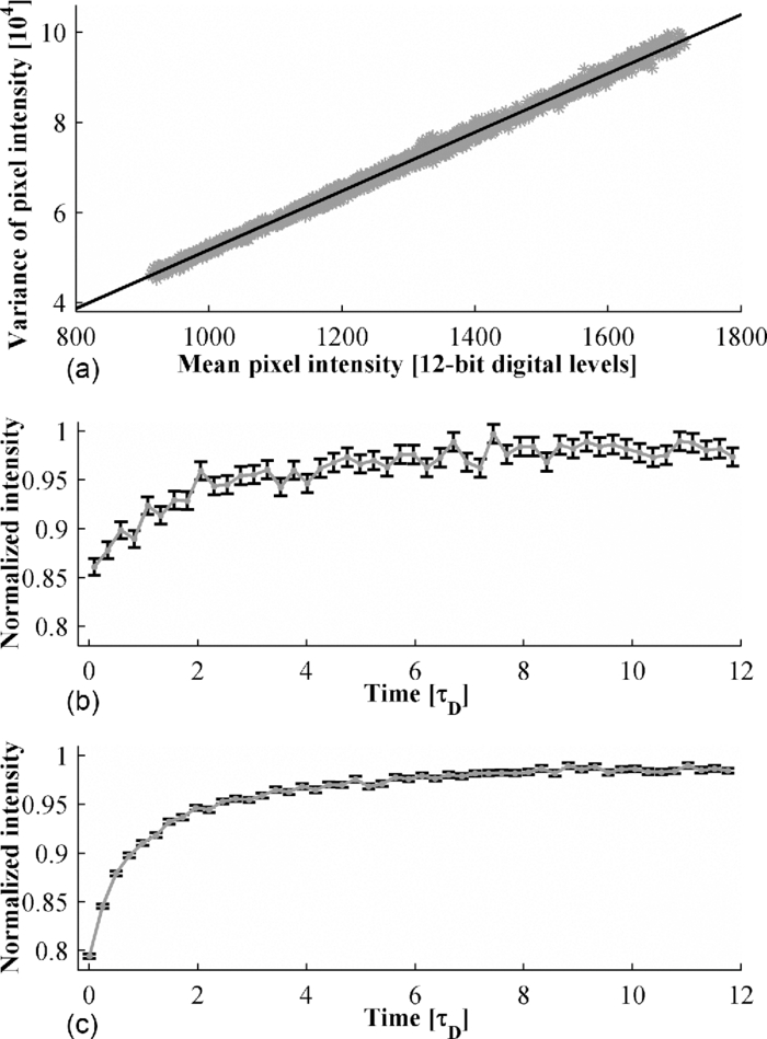

3.5.

Analysis of Recovery Curves

Each set of recovery curves was analyzed in two distinct ways. In the first approach, further referred to as single-curve analysis, each curve was separately analyzed utilizing the calibrated resolution parameters r _b and r _d. In the second approach, two global analyses of all recovery data were performed. These global analyses respectively utilized and ignored the calibrated values of the resolution parameters to investigate the feasibility of recovering the combined resolution parameter R [cf. Eq. 11] exclusively from the recovery data themselves.

In the single-curve analysis, each experimental recovery curve was fit to the UDM [Eq. 10] and to the new GDM [Eq. 11], both adjusted for a mobile fraction M through Eq. 12, using a weighted nonlinear least-squares optimization minimizing

For setup A, the photobleaching resolution r _b for both models was set to 2.5 μm: 2 μm as determined from lineFRAP experiments¹² increased with 0.5 μm to account for the 2-pixel rise time of the acousto-optical modulator (AOM). For setup B, r _b was set to 1.9 μm: 1.4 μm calibrated using lineFRAP [FD500 in 56% (w/w) sucrose, data not shown] increased with 0.5 μm analogously to setup A.

For the GDM, r _d was set to 1.0 and 0.9 μm for setups A and B, respectively. The mobile fraction M was set freely adjustable for consistency check: for the FITC-dextran solutions M should approximate 1. Results were grouped per ROI radius by calculating the weighted average values of the obtained parameter values.

For simultaneous analysis of a set of recovery curves, home-written routines were used. These routines make use of a nonlinear least-squares optimization algorithm. Parameters can be linked across recovery curves (i.e., made global) such that their values are equal for all selected recovery curves. Several sets of initial guesses were used to verify the true global minimum.

The obtained results were compared to the values obtained using the Stokes–Einstein equation

4.1.

Comparison of Uniform Disk Model to New Generalized Disk Model: Single-Curve Analysis

FD2000 solutions were used for setup A and FD500 solutions for setup B. The viscosity of the solutions was increased using different amounts of sucrose [40 and 56% (w/w)] to cover a range of diffusion coefficients (0.205–2.22 μm²/s). For a given viscosity, FRAP experiments were carried out on the same sample using photobleaching disks of varying radii. Hence, it was expected that all experiments would yield identical results.

Each experiment was analyzed by single-curve analysis using the classic UDM and the new GDM. Representative results are shown in Fig. 4. For all FRAP experiments analyzed, the mobile fraction M was close to 1 for both models, as expected from the model system used in these experiments. For setup A with r _b = 2.5 μm, it could be expected that for the UDM the calculated D values are independent of the radius for radii >10 μm (i.e., 4–5 times the effective photobleaching resolution). For smaller radii, D values recovered using the UDM were expected to gradually decrease because of the underestimation of the effective ROI size. For the smallest disk size, the UDM underestimates the expected diffusion coefficient by a factor of 2. On setup B, an entirely similar trend was observed, demonstrating that the deviations are not instrument related [Fig. 4b].

Fig. 4

Comparison of the UDM (empty squares) and the GDM (filled bullets). Representative data sets are shown for (a) setup A with FD2000 and (b) setup B with FD500 dissolved in, respectively, 56 and 40% (w/w) sucrose. Results are grouped per ROI radius using weighted averages of the obtained diffusion coefficient D. Number of recovery curves per ROI radius varied between 5 and 10. The UDM returned a diffusion coefficient that decreased with decreasing ROI radius, reaching a maximum underestimation at the smallest ROI size. Error bars are shown as standard deviations.

Analysis of the same data sets with the GDM nicely resulted in diffusion values that are independent of the disk size (within the experimental error). We note that small bleaching depths were used, K ₀ < 0.3, consistent with the linearization in Eq. 4. Thus, the underestimation of the effective radius of the ROI in the UDM was appropriately compensated by the new model. For large ROIs, the D values of the UDM asymptotically approach the values of the GDM, as can be expected.

4.2.

Comparison of Uniform Disk Model to New Generalized Disk Model: Global Analysis

Because all recovery curves in a data set are derived from the same sample, they are all characterized by the same diffusion coefficient D. This is often implemented in the data analysis by averaging over all measurements, either at the level of the recovery curves themselves or at the level of the measured D values. In the current paper, a third implementation is used: a simultaneous analysis with the parameter D linked across all related recovery curves (i.e., a single, global parameter for D shared by all recovery curves). Other parameters, such as the bleaching depth and the mobile fraction, can be kept local (i.e., these fitting parameters are specific for each individual recovery curve). This approach allows for differences in these parameters between recovery curves.

All data sets were analyzed using this global analysis applying both UDM and GDM. Similar to the single-curve analysis, the latter model made use of the calibrated resolution factor R by incorporating it as a fixed (i.e., nonadjustable) parameter. For all data sets globally analyzed, D recovered using the UDM was consistently smaller as compared to the GDM that better approached the theoretical expected value (Table 1). The uncertainties on these recovered values are similar for both models. The underestimation of D by the UDM, however, was smaller than observed using solely the smallest ROI size in the single-curve analysis. In other words, inclusion of large ROI sizes moderates the underestimation of D, as can be expected.

Fig. 6

Related data sets were repeatedly analyzed using global analysis while progressively including larger ROIs. D was linked across all included recovery curves. Representative data sets are shown obtained with FD2000 in (a) 40% and (b) 56% w/w sucrose/HEPES buffer using setup A. Error bars representing the standard deviations are shown if larger than the symbol size.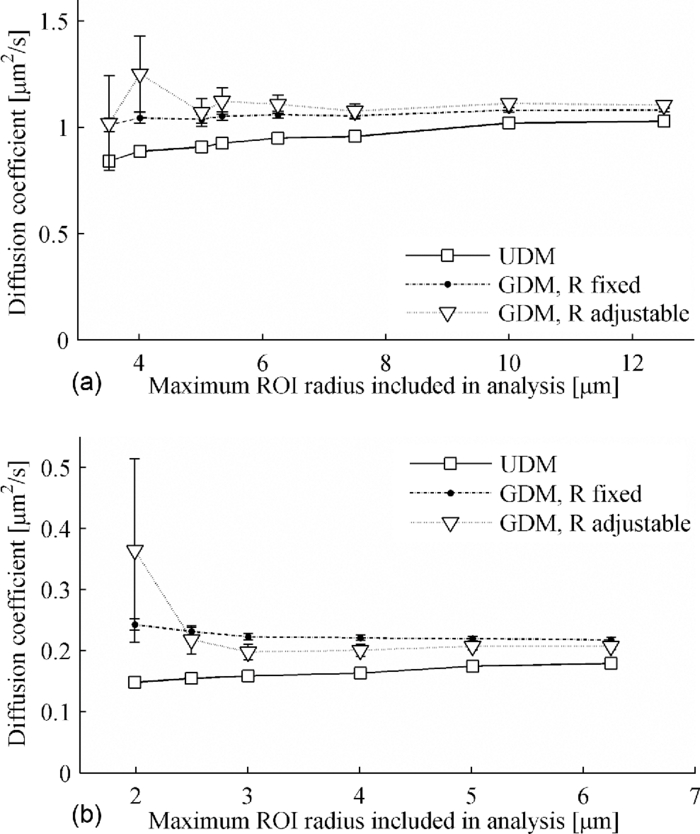

Table 1

Global analysis of FITC-dextran experiments for UDM and GDM at room temperature. Uncertainties are reported as standard deviations.

Single-curve analysis of FRAP data using the GDM requires a priori knowledge of r _d and r _b, which are combined in the parameter R. This means that R is kept constant and identical in the individual analysis of all related recovery curves. However, in a simultaneous analysis of related recovery curves arising from different ROI sizes, the common value of the parameter R can be determined by linking R over the related curves (i.e., there is a single parameter R in the optimization routine). Best results are obtained when R is linked across as many ROI sizes as possible.

This approach does yield D values close to the expected values (Table 1). Compared to the approach that applies a fixed R, the recovered values of D are identical within the experimental error and their uncertainties nearly double but remain of the same order of magnitude. In other words, even without making use of a priori information on, the correct D can be obtained when a range of ROI sizes is considered.

Since r _d is known, the r _b values can be calculated from the fitted R values. For all data sets analyzed, a physically relevant r _b value approaching the calibrated value is obtained (Table 2).

Table 2

Comparison of the calibrated bleach resolution r b to the recovered value from the global analyses using the obtained R and the calibrated value of r d.

4.3.

Importance of R per ROI Size

The correction factor R is more important with decreasing ROI radius (vide supra). To experimentally confirm this statement, the accuracy by which R can be determined per ROI size is investigated. R should be obtained with higher accuracy from small ROI radius as compared to their larger counterparts. This was investigated by linking D over all recovery curves and by linking R within experiments of the same ROI size. The recovered values of R displayed a variability among the different ROI sizes without significant differences (Fig. 5). It was obvious that the uncertainty on R increased with increasing ROI radius, thereby corroborating the theory.

Fig. 5

Resolution factor R as a function of ROI radius, recorded with setup A and FD2000 dissolved in 56% (w/w) sucrose in HEPES buffer. Error bars represent standard deviations.

4.4.

Effect of Omitting Large ROIs in Global Analysis

Analysis including recovery curves from all ROI sizes led to a reliable result. Experimental conditions, however, do not always allow for large ROIs in case of small samples. Therefore, it was necessary to investigate the performance of the new GDM with freely adjustable R when only these smaller sizes are considered. A global analysis was repeatedly performed starting with only the two smallest ROI sizes and progressively including larger ROI sizes. Figure 6 displays the results of two representative data sets obtained with FD2000 in 40% [Fig. 6a] and 56% [Fig. 6b] (w/w) sucrose using setup A and analyzed by the presented method.

Applying this strategy using UDM, it comes as no surprise that the obtained values for D using only small ROIs severely deviate from the expected value (Fig. 6). When larger ROIs were also included, D increased but never reached the expected value. With the GDM and a fixed value of R, on the other hand, the correct value of D could be found already with only two to three small ROI sizes at the expense of a larger uncertainty on the fitted parameters (Fig. 6). This conclusion was similar among all data sets, indicating that small ROIs are sufficient to accurately determine D.

A similar analysis was performed using GDM but with a linked R across the data as a free-fitting parameter. This approach yielded better D values than the UDM. In comparison to GDM with a fixed R, somewhat more variation in the recovered D values could be observed. Nevertheless, even without any prior knowledge of R, the GDM clearly outperforms the UDM.