|
|
1.IntroductionDiffuse optical tomography (DOT) is an emerging, noninvasive functional imaging modality that has demonstrated the clinical potential for distinguishing benign from malignant breast lesions 1, 2, 3, 4, 5, 6, 7, 8, 9, 10, 11, 12, 13, 14, 15 and for monitoring neoadjuvant chemotherapy response of advanced breast cancers. 16, 17, 18, 19, 20, 21, 22 In our study, we have used an ultrasound-guided DOT to overcome the limitation of inaccurate target quantification by DOT alone. Because commercial pulse-echo ultrasound is employed in reflection geometry, DOT is implemented in the same geometry for coregistration of both modalities. In the reflection-geometry DOT, the light sources and detectors are deployed on a handheld probe and data are acquired from the surface of the breast tissue. In DOT imaging reconstruction, born approximation is typically used to relate the unknown optical properties of the tissue to the measurements at the tissue surface and inversion is performed with the conjugate gradient iterative searching method. We have employed a semi-infinite absorbing boundary condition to derive the weight matrix, which describes the so-called banana-shaped path of light propagation for a given source and detector pair on the surface. Because the iterative searching method is highly prone to converge along the steepest direction, (i.e., the largest weight direction), this banana function causes the reconstructed optical properties to be depth dependent. As a result, even for a homogeneous large target, the reconstructed absorption coefficients of top target layers, which normally have more weight, are higher than those of the deeper target layers. This is an intrinsic problem related to light diffusion in the turbid medium. Therefore, it is essential to correct for the depth dependency of the weight matrix before starting the iterative searching procedure. In our previous study, we introduced a depth-correction method that incorporated the lesion depth information provided by coregistered ultrasound.23 Generally, using the prior information of the lesion location reduced the number of voxels with unknown optical properties; thus, the inversion converged in a few number of iterations. In that approach, the weight matrix was balanced by normalizing its elements to the maximum of each layer in depth, which improved the reconstruction for large phantom targets, but the procedure was ad hoc. A method of depth compensation based on the maximum singular values (MSVs) of the weight matrix in different depths, was recently introduced by Niu 24 In their method, due to the ill-conditioned inverse problem, a penalty term was added to the forward model to stabilize the solution. Therefore, the algorithm actually derived the result from an inaccurate forward model. As a result, another scaling parameter was estimated to obtain the original absorption map.25 In this study, we have adopted the MSV approach introduced by Niu,24 and appropriately scaled the weight matrix using the MSVs of the background and lesion layers indentified by coregistered ultrasound independently without changing the forward model. The inversion was performed using the scaled weight matrix, and the reconstructed absorption distribution was scaled back after inversion. This depth-correction procedure is precise, and no approximation is used. In this paper, the improvement of using this new depth-correction algorithm is quantitatively evaluated using phantom targets and 10 clinical cases of large malignant and benign lesions. 2.Methods2.1.Reconstruction Algorithm with Depth CorrectionIn our ultrasound-guided DOT image reconstruction, a dual-zone mesh scheme is used to segment the imaging volume into a lesion region, L, and a background region, B, with fine and coarse voxel sizes, respectively.26 The forward model based on the diffusion equation, linearized by modified born approximation, is written as follows: Eq. 1[TeX:] \documentclass[12pt]{minimal}\begin{document}\begin{equation} U_{{\rm sd}} = \left[ {W_{\rm L},W_{\rm B} } \right]\left[ {M_{\rm L}, M_{\rm B} } \right] \end{equation}\end{document}In Eq. 1, U sd is the scattered field measured at each source and detector pair, [M L, M B] denotes the total absorption distribution, and [W L, W B] denotes the weight matrix of lesion and background regions, respectively. Weight matrix describes the distribution of diffusive wave in the homogenous medium and characterizes the measurement sensitivity to the absorption changes in both spatial dimensions and in depth. For computing the weight matrix, we have used a semi-infinite absorbing boundary condition at the surface and the corresponding analytic solution of the diffusion equation. In addition, the average optical absorption and reduced scattering coefficient of the background medium needed for the weight matrix computation are obtained from the measurements made with the homogenous intralipid solution for phantom experiments and the normal contralateral breast for clinical study. Finally, after computing the weight matrix, inversion is performed with the conjugate gradient iteration searching method to obtain the total absorption map from Eq. 1 and the total distribution was divided by different voxel sizes at the lesion and background regions to obtain the absorption distribution. A proper scaling factor is required to balance the exponential decay of the weight matrix elements with depth. In general, singular value decomposition of a two-dimensional matrix, is intuitively interpreted as a sequence of three geometrical transformations: a rotation, a scaling, and another rotation. The scaling transformation is a diagonal matrix where the diagonal entries are matrix singular values. In addition, the Eckart–Young theorem states that the least-squares approximation in α dimension of a matrix of rank β can be found by replacing its smallest (α–β) singular values to zeroes.27 It means that the large singular values contain most of the information in a data matrix, and this is principally the basis of a method for compressing the information in a matrix. On the basis of these properties, the maximum singular value of a matrix has the maximum information related to the scaling performance of its elements. As a result, for correcting the depth dependency of the weight matrix, the MSV of the weight elements of each layer is used. Our modified algorithm for balancing the weight matrix using the MSVs of different depth layers, given the coregistered ultrasound information, is as follows. In the first step, the elements of weight matrix are grouped layer by layer from top to bottom in the lesion and background regions as [TeX:] $[W_{\rm L},W_{\rm B}]\break = [(W_{\rm L}^1,\ldots,W_{\rm L}^n),(W_{\rm B}^1,\ldots,W_{\rm B}^m)]$ , where [TeX:] $W_{\rm L}^i,i = 1,\ldots,n$ represent the weights of voxels of the i’th layer of lesion region with n layers, and [TeX:] $W_{\rm B}^j,j = 1,\ldots,m$ represents weights of voxels of the j’th layer of background region with m layers. Then a scaling diagonal matrix including the MSVs of the layers is composed as [TeX:] $[S_{\rm L},S_{\rm B}] = [{\rm diag}(\lambda _{\rm L}^n,\ldots,\lambda _{\rm L}^1),{\rm diag}(\lambda _{\rm B}^m,\ldots,\lambda _{\rm B}^1)]$ , where [TeX:] $\lambda _{\rm L}^i$ is the MSV of the i’th layer of the lesion region, and [TeX:] $\lambda _{\rm B}^j$ is the MSV of the j’th layer of the background. Note that the MSVs are rearranged inversely in the order from bottom to top layer in both regions to compensate the decrease of the photon density with depth at the next step. Then, the forward model is rewritten as follows: Eq. 2[TeX:] \documentclass[12pt]{minimal}\begin{document}\begin{eqnarray} U_{{\rm sd}} &=& ({[ {W_{\rm L}, W_{\rm B} } ][ {S_{\rm L},S_{\rm B} } ]})({[ {S_{\rm L},S_{\rm B} } ]^{ - 1} [ {M_{\rm L}, M_{\rm B} } ]})\nonumber\\ &=& \left[ {W_{\rm L}, W_{\rm B} } \right]^{\prime \prime } \left[ {M_{\rm L}, M_{\rm B} } \right]^{\prime \prime }. \end{eqnarray}\end{document}Consequently, by applying the new weight matrix multiplied by the scaling matrix, W ″, in the iterative inversion, depth dependency of the reconstructed layers is relatively compensated. Finally, the result of the inversion is scaled with the same scaling matrix to obtain the original total absorption map of [M L, M B] = [S L, S B][M L, M B]′′. 2.2.Phantom and Clinical ExperimentsThe experiments were performed with our frequency domain near infrared (NIR) system that consisted of source and detection subsystems as well as a handheld probe.26 The source has four laser diodes of wavelengths 740, 780, 808, and 830 nm. In this study, the measurements obtained from 780-nm laser diode was used because an optical absorption map was reconstructed to demonstrate the depth correction approach. Each – laser diode was modulated at 140 MHz and sequentially coupled into nine optical source fibers through 4×1 and 1×9 optical switches. The reflected light from tissue associated with each of the illumination source was detected with 14 optical fiber bundles of 3 mm diam, simultaneously. The detection fibers coupled the light into 14 parallel photomultiplier tubes and electronics channels. The configuration of the source and detector fibers distributed on the handheld probe with a coregistered ultrasound transducer in the middle, is shown in Fig. 1. Fig. 1Configuration of source and detector optical fibers distributed on the handheld probe. The source and detector locations are shown with stars and circles, respectively. A commercial ultrasound transducer is located in the middle open slot. 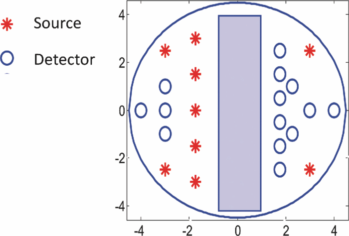 In phantom experiments, 0.8% intralipid solution emulated the background breast tissue optical properties with the calibrated absorption coefficient μa in the range of 0.02–0.03 cm−1 and reduced scattering coefficient [TeX:] $\mu ^{\prime} _{\rm s}$ in the range of 6.9–7.8 cm−1. The solid plastisol phantoms with the calibrated optical properties of μa = 0.158 cm−1, [TeX:] $\mu ^{\prime} _{\rm s} = 6.53\ {\rm cm}^{ - {\rm 1}}$ , and μa = 0.075 cm−1, [TeX:] $\mu ^{\prime} _{\rm s} = 5.6\ {\rm cm}^{ - {\rm 1}}$ were used to model the high- and low-contrast lesions, respectively. The optical reflectance data of the phantom submerged in the intralipid at different depths were acquired with the NIR system, while the coregistered ultrasound provided the location information. The surface of the handheld probe was considered as the reference plane for the depth measurement. Figure 2 displays different types of phantoms used in the reported experiments, including homogenous high-contrast (HH), homogenous low-contrast (HL), top high-contrast (TH), and top low-contrast (TL) targets. Each of the homogenous and non-homogenous phantoms shown in Fig. 2 had two sizes of diameter, 2 and 3 cm. The imaging volume considered in the reconstruction was 8 × 8 × 4 cm3. The voxel sizes of 0.25 × 0.25 × 0.25 cm3, and 1.5 × 1.5 × 1.5 cm3 were applied to the lesion and background regions in x-y-z plane, respectively. Fig. 2Experimental phantoms of (a) homogenous high contrast (HH), (b) homogenous low contrast (HL), (c) top high contrast (TH), and (d) top low contrast (TL).  For the clinical studies, the protocol is approved by the local Institution Review Board and all patients signed the informed consent. Patients were scanned in a supine position while multiple sets of optical reflectance measurements were made with coregistered ultrasound images at the lesion location and the normal contralateral location of the same quadrant as the lesion. As mentioned in Sec. 2, the optical properties of the background required for computing the weight matrix were estimated from measurements obtained at the normal contralateral location. 2.3.Evaluation of Reconstructed ImagesThe performance of the depth-correction method is evaluated using phantom targets and clinical cases. To quantitatively compare the results without and with the correction method, the reconstructed absorption maps for each type of lesion shown in Fig. 2 are given in Sec. 3. The spatial map in the x-y plane is shown with 0.5- and 0.25-cm increments in depth for the phantom lesions and clinical cases, respectively. To further quantify the improvement with the correction method, maximum absorptions of the layers in the lesion region are extracted from the corresponding reconstructed absorption maps. The standard box and whisker plots of this data are presented, in which the first and third quartiles of data are at the ends of the box, the median is indicated with a vertical line in the interior of the box, and the maximum and minimum values are at the ends of the whiskers.28 The location of the box within the whisker provides insight on the data distribution that implies the depth sensitivity in our case. Normally, the maximum reconstructed absorption is comparable to the true value. Therefore, improving depth sensitivity mainly raises the recovered values of deeper layers of a homogenous lesion. This effect is indicated in the plots by the increase of the median or shift of the box toward the maximum level. Furthermore, the box size is related to the data variation such that the smaller box size is due to the smaller absorption variation inside the lesion region. The other factor calculated for homogenous cases is the position error (PE), defined as the absolute difference between the depth of the maximum reconstructed absorption and the true depth of the lesion center. To quantify the accuracy of characterization of the nonhomogenous phantoms, the ratio of the absorption is calculated in lesion region as defined by Eq. 3[TeX:] \documentclass[12pt]{minimal}\begin{document}\begin{equation} R = \frac{{{\rm Max\, absorption\, of\, top\, half}}}{{{\rm Max\, absorption\, of\, bottom\, half}}}. \end{equation}\end{document}The expected values of this ratio are R = 1 for the homogenous phantoms, R = 2 for TH contrast, and R = 0.5 for TL contrast phantoms. 3.Results3.1.Homogenous Phantom ExperimentsThe absorption map of the high- and low-contrast homogenous phantoms of 2 cm diam, reconstructed without and with using the depth correction is shown in Fig. 3. The slices in each panel showing the spatial map in x-y plane at depths of 0.5–3 cm with 0.5-cm increments. The phantom center is located at depth of 2 cm, measured from the probe surface. Without depth correction, the top layer at depth of 1.25 cm has the maximum absorption of 0.1345 for the HH phantom and 0.104 for the HL one, which are about 84 and 72% of the expected values. With depth correction, the center layer at depth of 2 cm has the maximum absorption of 0.1356 for HH and 0.102 for HL phantom, which are about 85 and 73% of the expected values. Although the reconstructed maximum absorption values are similar before and after correction, the target mass is reconstructed at the center depth rather than at the top portion of the target. Fig. 3Reconstructed absorption map of a homogenous phantom of 2 cm diam with the center located at depth of 2 cm. (a, b) High-contrast phantom without and with depth correction, respectively; (c, d) low-contrast phantom without and with depth correction, respectively. Each image consists of six subimages. Each subimage is the spatial x-y image of 8×8 cm reconstructed at the depth marked on its title. The increment in depth is 0.5 cm. For the absorption maps reported in this paper, the spatial dimensions of the subimage were kept the same and the reconstruction depth might be different based on the target location.  The same experiment was performed for the HH and HL phantoms of 2 cm diam located at depths of 1.5, 2.5, and 3 cm, in addition to the HH and HL phantoms of 3 cm diam located at depths of 2, 2.5, and 3 cm. For all cases, the maximum absorptions of target layers were extracted from the reconstructed maps. Then, the box and whisker plots for that data are presented in Figs. 4, 5. These box plots show that the median of the reconstructed absorption inside the phantoms increased toward the maximum absorption after applying depth correction. This improvement is calculated for all phantoms, and the result is listed in Table 1. It is seen that the median is closer to the maximum for the HL phantoms in comparison to HH phantoms of the same size. It is also demonstrated in the box plots that the box size reduced due to applying depth correction. This confirms the decrease of the absorption variation inside the homogenous phantoms. The box-size reduction on average is about two times for the 2-cm-diam targets and 1.8 times for the 3-cm-diam ones. In general, the box size increases with increasing depth, while it is more consistent by applying the depth correction, indicating more uniform depth sensitivity. Overall, the boxes of the bigger phantoms are larger that demonstrate the increase of absorption variation inside the larger phantoms. It is also represented in Figs. 5b and 5d that, unlike the HH cases shown in Fig. 4, the depth sensitivity is increased for the bottom layers of HL phantoms located at depth of 3 cm. Fig. 4The box and whisker plot of the maximum absorption of the layers in the lesion region. Homogenous high contrast of size 2 cm diam reconstructed (a) without and (b) with depth correction. Homogenous high-contrast lesion of size 3 cm diam reconstructed (c) without and (d) with depth correction. 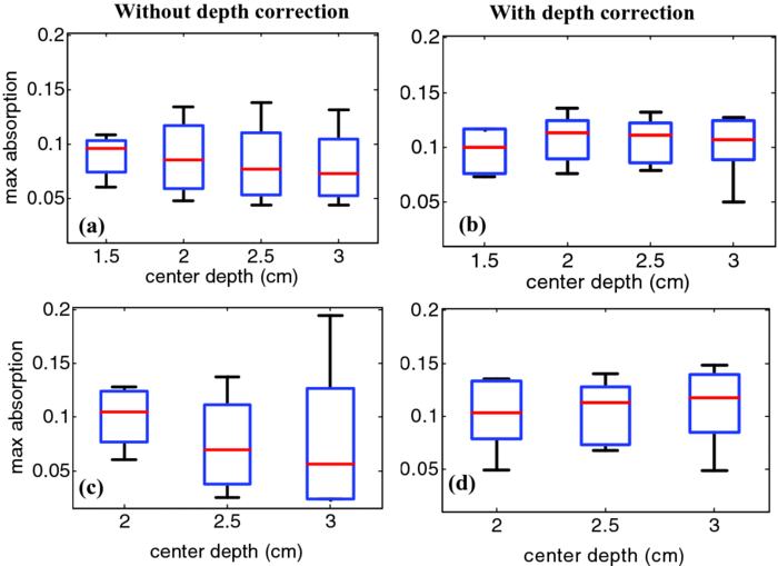 Fig. 5The box and whisker plot of the maximum absorption of the layers in the lesion region. Homogenous low-contrast lesion of size 2 cm diam reconstructed (a) without and (b) with depth correction. Homogenous low-contrast lesion of size 3 cm diam reconstructed (c) without and (d) with depth correction. 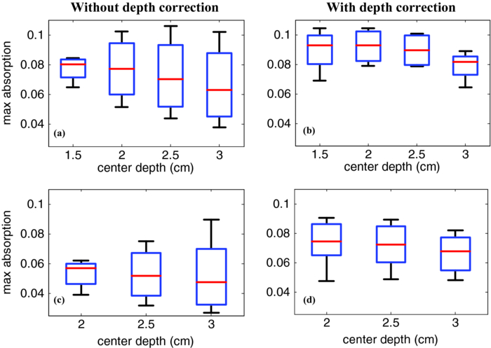 Fig. 10The box and whisker plot of the maximum absorption of the layers in the lesion region. Malignant cases reconstructed (a) without and (b) with depth correction. Benign cases reconstructed (c) without and (d) with depth correction.  Table 1Compare the median of the data in the lesion layers to its maximum absorption reconstructed without and with depth correction.
Lastly, the PE is evaluated for all cases. The error is in the range of the phantom radius, i.e., 0.75 cm for 2-cm-diam phantoms and 1.25 cm for the 3-cm-diam ones that decreases to the range of the reconstruction mesh sizes, i.e., 0.25 cm after using depth correction. 3.2.Nonhomogenous Phantom ExperimentsThe TH and TL phantoms of 2 cm diameter, located at depth of 2 cm are also imaged. The maximum reconstructed absorption of TH phantom is 0.152 cm−1 at 1.25-cm depth while it has moved to the depth of 1.75 cm with the value of 0.13 cm−1 by using the depth-correction method. For the TL phantom, there is no information from the bottom half of the target when the reconstruction is performed without depth correction. The maximum absorption of 0.059 cm−1 is measured at the top layer at a depth of 1.25 cm, whereas with depth correction, the maximum absorption is 0.073 cm−1 at a depth of 2.25 cm. Figures 6a and 6b show the depth profiles from 0.5 to 3.5 cm, of four types of phantoms. All of them are 2 cm diam in size and are located at a depth of 2 cm. After applying depth correction, the maximum reconstructed absorption is at the center mass for the homogenous cases, whereas it is located at top of the center line for the TH phantom and below the center line for the TL one. Hence, it is clearly indicated in Fig. 6b that the phantoms can be more accurately characterized. In order to quantify this effect, the ratio R is calculated for the phantoms of 2 cm in size located at different depths and the results are shown in Table 2. It is seen that R is always >1 for the reconstructions without depth correction because the maximum absorption is always at the top layer. Whereas, by applying depth correction, R gets closer to the expected values for the targets located at depths up to 2.5 cm. At a depth of 3 cm, the bottom half value is close to the background value and R is still >1 for the TL case. Therefore, with the threshold of R = 1, different types of the phantoms are almost precisely characterized. The same factor, R, is calculated for the phantoms of 3 cm in size, and the results are listed in Table 3. Comparing the result without and with depth correction confirms the improvement in the ratio by applying the correction method for the targets located at a depth of 2 cm. At a depth of 2.5 cm, the ratio calculated for HH target is >1 and is very close to 1 for the TL phantom. Therefore, the threshold of R = 1 was not successful for these cases. Fig. 6Depth profiles of reconstructed absorption map (a) without and (b) with depth correction for top low-, homogenous low-, homogenous high-, and top high-contrast, 2-cm-diam phantoms located at a depth of 2 cm from left to right.  Table 2Ratio of maximum absorption of the top half to the maximum absorption of the bottom half, R, calculated for phantoms of 2 cm diam, reconstructed without (w/o) and with (w) using depth correction.
Table 3The ratio of maximum absorption of top half to the maximum absorption of bottom half, R, calculated for phantoms of 3cm diam that were reconstructed without (w/o) and with (w) using depth correction.
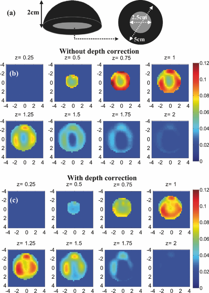
Before applying the correction to the clinical cases, it is necessary to study its effect on the known inhomogeneous phantom. This experiment was performed for the plastisol phantom shown in Fig. 7a. The middle core had a low contrast half-sphere of 2.5 cm diam embedded in the high-contrast shell phantom of 5 cm diam and height of 2 cm. The absorption coefficient was μa = 0.25 cm−1 for the outer shell and μa = 0.06 cm−1 for the core. The distance between the bottom of the phantom and the probe surface was 2.3 cm. The result of reconstruction, shown in Figs. 7b and 7c, verified that the depth-correction method kept the inhomogeneous target profile while enforcing better sensitivity for deeper layers. It also shifted the reconstructed maximum absorption of 0.139 cm−1 at a depth of 0.75 cm to the location of central mass at 1.25-cm depth with a maximum absorption coefficient of 0.11 cm−1. 3.3.Clinical StudiesThe absorption maps of benign and malignant large lesions reconstructed without and with depth correction are evaluated in this section. Figure 8a shows a coregistered ultrasound B-scan of a larger suspicious mass located at 10 o'clock position of the right breast of a 43-year-old woman. The large lesion region is marked with the white dashed line. The borders of the lesion were not clear, and the size estimated by ultrasound was about 3×3 cm in spatial dimensions and 2.0 cm in depth. The fitted background tissue optical properties were μa = 0.23 cm−1 and [TeX:] $\mu ^{\prime} _{\rm s} = 2.12\ {\rm cm}^{ - 1}$ . The core needle biopsy revealed that the lesion was an invasive ductal carcinoma. Figures 8b and 8d illustrate the reconstructed absorption maps at depth of 0.5–3 cm with 0.25-cm increments, and Figures 8c and 8e show the reconstructed absorption profiles in depth. Similarly, Fig. 9 shows a coregistered ultrasound and the absorption maps of a large suspicious lesion located at 8 o'clock position of the right breast of a 39-year-old woman. The borders of the lesion were not clear and the estimated dimensions by ultrasound were 5 × 5 cm in spatial dimensions and 2.2 cm in depth. The calibrated optical background was μa = 0.03 cm−1 and [TeX:] $\mu ^{\prime} _{\rm s} = 5.93\;{\rm cm}^{ - 1}$ . The core needle biopsy revealed that the lesion was a benign fibrocystic change with a moderate degree of intraductal hyperplasia. For the malignant case, the maximum absorption was 0.44 cm−1 at a depth of 1.25 cm that was shifted to the depth of 1.75 cm with the value of 0.37 cm−1. For the benign case, the maximum was 0.11 cm−1 at a depth 1.25 cm that moved to 2.25 cm with the value of 0.118 cm−1 after using depth correction. Fig. 9A benign lesion obtained from a 39-year old woman. (a) A coregistered ultrasound B-scan. (b, c) Reconstructed absorption maps in (b) spatial and (c) depth without depth correction. (d, e) Absorption maps with depth correction.  The box and whisker plot of the maximum absorption of the lesion layers for 10 larger lesions, including five benign and five malignant cases, is shown in Fig. 10. Table 4 provides patient information, lesion size, and center depth as measured by coregistered ultrasound. The box size reduction is ∼2.7 times for malignant cases and two times for the benign ones. The median is 76 and 87% of the maximum value that improves to 96 and 98% after depth correction used for the malignant and benign lesions, respectively. Note that, the benign lesions in general have smaller box size than the malignant ones. Table 4Patient information and lesion location size and center depth measured by coregistered ultrasound.
4.Discussion and SummaryIn this study, we have introduced a depth-correction method that balances the weight matrix at the typical depth range encountered in the breast imaging of large lesions in the reflection geometry. Another factor that contributes to the depth-dependent absorption mapping in addition to the weight matrix, is the light-shadowing effect caused by highly vascularized tumors.29 The significant absorption of a tumor causes a dramatic reduction of the reflected light received from the deeper portion of the tumor. As a result, the lower portion of the lesion is not quantified correctly. This posterior light-shadowing effect is similar to the sound-shadowing effect frequently seen in pulse-echo ultrasound images. The presence of significant posterior shadowing of a lesion in ultrasound images suggests malignance. As an example, the malignant case shown in Fig. 8 revealed much higher absorption with maximum located at the top target layer, which moved 0.25–0.5 cm deeper after depth correction. However, the high-absorption layers were still at the top part of the tumor mass. As seen by ultrasound, the tumor mass center was approximately located at 2-cm depth. For the benign case seen in Fig. 9, the higher absorption was also shown at the top target layer and it was moved to approximately the center of the mass after applying the correction. This suggests that the shadowing effect is more pronounced for the malignant case and is not compensated after applying the depth correction. Fig. 8A malignant cancer obtained from a 43-year-old woman. (a) A coregistered ultrasound B-scan. The cancer was located from 1 to 3 cm in depth. (b, c) Reconstructed absorption maps in (b) spatial and (c) depth without depth correction. (d, e) Absorption maps with depth correction. 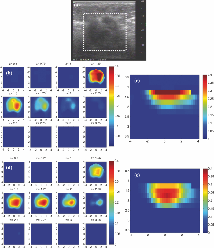 In Ref. 29, we derived a simple measure to quantify the effect of light shadowing due to optical contrast only. The measure is obtained from a pair of high- and low-contrast targets of a similar size, a similar target location, and similar background optical properties. This measure is defined as shadowing factor = ratio of reconstructed maximum μa measured at the highest absorption layer (depth) to that measured at the next deeper layer (depth) of a high-contrast lesion over the ratio similarly calculated from a low-contrast lesion. Therefore, this shadowing factor is independent from depth-dependent reconstruction caused by an unbalanced weight matrix, and it only depends on the optical contrast. Using the reported depth-correction method, the depth dependency due to the weight matrix distribution is compensated to a large extent and the shadowing effect can be used for characterizing the lesions individually. It is expected that for the benign lesions, the ratio of the maximum absorption of the highest absorption layer to that of the next deeper layer is close to unity because the reconstructed absorption map of the low contrast lesion after correcting unbalanced weight matrix is more uniform. Therefore, using depth correction, the malignant lesions can be directly characterized by using the ratio of the maximum absorption of the highest absorption layer over that measured at the next deeper layer. This ratio can be used directly without requiring a pair of lesions of similar size and location. For this small group of malignant and benign cases, the shadowing factor was measured using lesions of the similar size located at a depth of 2 cm (Table 4). Before depth correction, the ratio of the maximum absorption of the top layer to the maximum absorption of the next deeper layer is about two times for the malignant and ∼1.33 times for the benign cases. As a result, the shadowing factor is ∼1.5. After depth correction, the ratio of the maximum absorption of the highest absorption layer over the maximum absorption of the next deeper layer is 1.04 for benign cases and 1.3 for the malignant ones. This has resulted in a shadowing factor of 1.3, which is more accurate because the depth dependency of the weight matrix is corrected. This result is significant for accurate diagnosis of large malignant versus benign lesions once it is validated by more clinical cases. In summary, we have introduced a new depth-correction method that incorporates the target-depth information provided by coregistered ultrasound. This method balances the weight matrix by using the maximum singular values of the target layers in depth without changing the forward model. The performance of the method is evaluated using phantom targets and 10 clinical cases of larger malignant and benign lesions. The results for the homogenous targets demonstrate that the maximum absorption location error is reduced to the range of the reconstruction mesh size. Furthermore, the uniformity of absorption distribution inside the lesions has improved about two times and the median of absorption has increased from 60 to 85% of its maximum compared to no depth compensation. Clinical examples have showed a similar trend as phantom results and demonstrated the utility of the correction method for improving lesion quantification. AcknowledgmentsThe authors acknowledge funding support of this work from the National Institute of Health (Grant No. R01EB002136) and the Donaghue Medical Research Foundation. ReferencesD. R. Leff, O. J. Warren, L. C. Enfield, A. Gibson, T. Athanasiou, D. K. Patten, J. Hebden, G. Z. Yang, and
A. Darzi,
“Diffuse optical imaging of the healthy and diseased breast: a systematic review,”
Breast Cancer Res. Treat., 108
(1), 9
–22
(2008). https://doi.org/10.1007/s10549-007-9582-z Google Scholar
B. Chance, S. Nioka, J. Zhang, E. F. Conant, E. Hwang, S. Briest, S. G. Orel, M. D. Schnall, and
B. J. Czerniecki,
“Breast cancer detection based on incremental biochemical and physiological properties of breast cancers: a six-year, two-site study,”
Acad. Radiol., 12 925
–933
(2005). https://doi.org/10.1016/j.acra.2005.04.016 Google Scholar
S. P. Poplack, T. D. Tosteson, W. A. Wells, B. W. Pogue, P. M. Meaney, A. Hartov, C. A. Kogel, S. K. Soho, J. J. Gibson, and
K. D. Paulsen,
“Electromagnetic breast imaging: results of a pilot study in women with abnormal mammograms,”
Radiology, 243 350
–359
(2007). https://doi.org/10.1148/radiol.2432060286 Google Scholar
E. Heffer, V. Pera, O. Schütz, H. Siebold, and
S. Fantini,
“Near-infrared imaging of the human breast: complementing hemoglobin concentration maps with oxygenation images,”
J. Biomed. Opt., 9 1152
–1160
(2004). https://doi.org/10.1117/1.1805552 Google Scholar
X. Liang, Q. Zhang, C. Li, S. R. Grobmyer, L. L. Fajardo, and
H. Jiang,
“Phase-contrast diffuse optical tomography 1: pilot results in the breast,”
Acad. Radiol., 15
(7), 859
–866
(2008). https://doi.org/10.1016/j.acra.2008.01.028 Google Scholar
X. Intes,
“Time-domain optical mammography SoftScan: initial results,”
Acad. Radiol., 12
(8), 934
–947
(2005). https://doi.org/10.1016/j.acra.2005.05.006 Google Scholar
L. Spinelli, A. Torricelli, A. Pifferi, P. Taroni, G. Danesini, and
R. Cubeddu,
“Characterization of female breast lesions from multiwavelength time-resolved optical mammography,”
Phys. Med. Biol., 50 2489
–2502
(2005). https://doi.org/10.1088/0031-9155/50/11/004 Google Scholar
C. H. Schmitz, D. P. Klemer, R. Hardin, M. S. Katz, Y. Pei, H. L. Graber, M. B. Levin, R. D. Levina, N. A. Franco, W. B. Solomon, and
R. L. Barbour,
“Design and implementation of dynamic near-infrared optical tomographic imaging instrumentation for simultaneous dual-breast measurements,”
Appl. Opt., 44 2140
–2153
(2005). https://doi.org/10.1364/AO.44.002140 Google Scholar
A. Athanasiou, D. Vanel, C. Balleyguier, L. Fournier, M. C. Mathieu, S. Delaloge, and
C. Dromain,
“Dynamic optical breast imaging: a new technique to visualise breast vessels: comparison with breast MRI and preliminary results,”
Eur. J. Radiol., 54
(1), 72
–79
(2005). https://doi.org/10.1016/j.ejrad.2004.11.022 Google Scholar
D. Floery, T. H. Helbich, C. C. Riedl, S. Jaromi, M. Weber, S. Leodolter, and
M. H. Fuchsjaeger,
“Characterization of benign and malignant breast lesions with computed tomographic laser mammography (CTLM),”
Investigat. Radiol., 40 328
–335
(2005). https://doi.org/10.1097/01.rli.0000164487.60548.28 Google Scholar
D. Grosenick, K. T. Moesta, M. Möller, J. Mucke, H. Wabnitz, B. Gebauer, C. Stroszczynski, B. Wassermann, P. M. Schlag, and
H. Rinneberg,
“Time-domain scanning optical mammography: I. recording and assessment of mammograms of 154 patients,”
Phys. Med. Biol., 50
(11), 2429
–2449
(2005). https://doi.org/10.1088/0031-9155/50/11/001 Google Scholar
B. Brooksby, B. W. Pogue, S. Jiang, H. Dehghani, S. Srinivasan, C. Kogel, T. D. Tosteson, J. Weaver, S. P. Poplack, and
K. D. Paulsen,
“Imaging breast adipose and fibroglandular tissue molecular signatures by using hybrid MRI-guided near-infrared spectral tomography,”
Proc. Natl. Acad. Sci. U S A, 103 8828
–8833
(2006). https://doi.org/10.1073/pnas.0509636103 Google Scholar
Q. Zhang, T. J. Brukilacchio, A. Li, J. J. Stott, T. Chaves, E. Hillman, T. Wu, M. A. Chorlton, E. Rafferty, R. H. Moore, D. B. Kopans, and
D. A. Boas,
“Coregistered tomographic x-ray and optical breast imaging: initial results,”
J. Biomed. Opt., 10 024033
(2005). https://doi.org/10.1117/1.1899183 Google Scholar
Q. Zhu, M. Huang, N. Chen, K. Zarfost, B. Jagjivant, M. Kane, P. Hedget, and
S. H. Kurtzmant,
“Ultrasound-guided optical tomographic imaging of malignant and benign breast lesions: initial clinical results of 19 cases,”
Neoplasia, 5 379
–388
(2003). http://www.ncbi.nlm.nih.gov/pubmed/14670175 Google Scholar
Q. Zhu, E. B. Cronin, A. A. Currier, H. S. Vine, M. Huang, N. Chen, and
C. Xu,
“Benign versus malignant breast masses: optical differentiation with US-guided optical imaging reconstruction,”
Radiology, 237 57
–66
(2005). https://doi.org/10.1148/radiol.2371041236 Google Scholar
Q. Zhu, P. Hegde, A. Ricci Jr., M. Kane, E. Cronin, Y. Ardeshirpour, C. Xu, A. Aguirre, S. Kurtzman, P. Deckers, and S. Tannenbaum,
“The potential role of optical tomography with ultrasound localization in assisting ultrasound diagnosis of early-stage invasive breast cancers,”
Radiology, 256 367
–378
(2010). https://doi.org/10.1148/radiol.10091237 Google Scholar
B. J. Tromberg, A. Cerussi, N. Shah, M. Compton, A. Durkin, D. Hsiang, J. Butler, and
R. Mehta,
“Imaging in breast cancer: diffuse optics in breast cancer: detecting tumors in pre-menopausal women and monitoring neoadjuvant chemotherapy,”
Breast Cancer Res., 7
(6), 279
–285
(2005). https://doi.org/10.1186/bcr1358 Google Scholar
R. Choe, A. Corlu, K. Lee, T. Durduran, S. D. Konecky, M. Grosicka-Koptyra, S. R. Arridge, B. J. Czerniecki, D. L. Fraker, A. Demichele, B. Chance, M. A. Rosen, and
A. G. Yodh,
“Diffuse optical tomography of breast cancer during neoadjuvant chemotherapy: a case study with comparison to MRI,”
Med. Phys., 32 1128
–1139
(2005). https://doi.org/10.1118/1.1869612 Google Scholar
H. Soliman, A. Gunasekara, M. Rycroft, J. Zubovits, R. Dent, J. Spayne, M. J. Yaffe, and
G. J. Czarnota,
“Functional imaging using diffuse optical spectroscopy of neoadjuvant chemotherapy response in women with locally advanced breast cancer,”
Clin. Cancer Res., 16
(9), 2605
–2614
(May 2010). https://doi.org/10.1158/1078-0432.CCR-09-1510 Google Scholar
Q. Zhu, S. Tannenbaum, P. Hegde, M. Kane, C. Xu, and
S. H. Kurtzman,
“Noninvasive monitoring of breast cancer during neoadjuvant chemotherapy using optical tomography with ultrasound localization,”
Neoplasia, 10
(10), 1028
–1040
(2008). https://doi.org/10.1593/neo.08602 Google Scholar
A. Cerussi, D. Hsiang, N. Shah, R. Mehta, A. Durkin, J. Butler, and
B. J. Tromberg,
“Predicting response to breast cancer neoadjuvant chemotherapy using diffuse optical spectroscopy,”
Proc. Natl. Acad. Sci. U S A, 104 4014
–4019
(2007). https://doi.org/10.1073/pnas.0611058104 Google Scholar
S. Jiang, B. Pogue, C. Carpenter, S. Poplack, W. Wells, C. Kogel, J. Forero, L. Muffly, G. Schwartz, K. Paulsen, P. Kaufman,
“Evaluation of breast tumor response to neoadjuvant chemotherapy with tomographic diffuse optical spectroscopy: case studies of tumor region-of-interest changes,”
Radiology, 252 551
–560
(2009). https://doi.org/10.1148/radiol.2522081202 Google Scholar
M. Huang and
Q. Zhu,
“Dual-mesh optical tomography reconstruction method with a depth correction that uses a priori ultrasound information,”
Appl. Opt., 43 1654
–1662
(2004). https://doi.org/10.1364/AO.43.001654 Google Scholar
H. Niu, F. Tian, Z. J. Lin, and
H. Liu,
“Development of a compensation algorithm for accurate depth localization in diffuse optical tomography,”
Opt. Lett., 35
(3), 429
–431
(2010). https://doi.org/10.1364/OL.35.000429 Google Scholar
F. Tian, H. Niu, S. Khadka, Z. J. Lin, and
H. Liu,
“Algorithmic depth compensation improves quantification and noise suppression in functional diffuse optical tomography,”
Biomed. Opt. Express, 1 441
–452
(2010). https://doi.org/10.1364/BOE.1.000441 Google Scholar
Q. Zhu, C. Xu, P. Guo, A. Aguirre, B. Yuan, F. Huang, D. Castilo, J. Gamelin, S. Tannenbaum, M. Kane, P. Hegde, and
S. Kurtzman,
“Optimal probing of optical contrast of breast lesions of different size located at different depths by U.S. localization,”
Technol. Cancer Res. Treat., 5
(4), 365
–380
(2006). http://www.ncbi.nlm.nih.gov/pubmed/16866567 Google Scholar
C. Eckart, G. Young,
“The approximation of one matrix by another of lower rank,”
Psychometrika, 1
(3), 211
–8
(1936). https://doi.org/10.1007/BF02288367 Google Scholar
R. McGill, J. W. Tukey and
W. A. Larsen,
“Variations of Boxplots,”
The American Statistician., 32
(1), 12
–16
(1978). https://doi.org/10.2307/2683468 Google Scholar
C. Xu and
Q. Zhu,
“Light shadowing effect of large breast lesions imaged by optical tomography in reflection geometry,”
J. Biomed. Opt., 15 036003
(2010). https://doi.org/10.1117/1.3431086 Google Scholar
|
|||||||||||||||||||||||||||||||||||||||||||||||||||||||||||||||||||||||||||||||||||||||||||||||||||||||||||||||||||||||||||||||||||||||||||||||||||||||||||||||||||||||||||||||||||||||||||||||||