|
|
1.IntroductionAccurate measurement of the physical and optical properties of the crystalline lens is essential in understanding the condition of presbyopia which is characterized by the gradual age-related loss of accommodation. These lens properties are closely related to each other, i.e., changes in the physical properties can result in changes in the optical properties.1 According to the Helmholtz theory of accommodation, contraction of the ciliary muscle releases tension on the zonules and the lens capsule causing the elastic lens capsule to mold the crystalline lens into a more spherical shape which increases its optical power. In the presbyopic eye, the gradual hardening of the lens contents reduces the ability of the lens to change shape and optical power. As a result, focusing on near objects is compromised. Using various imaging techniques, many previous models have been developed to understand and describe the shape and optical properties of the crystalline lens, both in vivo and in vitro. These techniques include the use of Purkinje images,2, 3 Scheimpflug photography,2, 4, 5 shadow photogrammetry,6 ultrasonography,7 and magnetic resonance imaging (MRI).4, 5, 8 A more recent imaging technique, optical coherence tomography (OCT), which was first demonstrated by Fujimoto 9 in 1991, has found wide spread use for high-resolution ocular imaging, from the corneal shape through to the retinal structure. This nondestructive, depth-penetrating technique is also useful to obtain cross-sectional and 3D images of the crystalline lens in vivo,10, 11 as well as ex vivo. 12 Most images of the lens require some form of adjustment to correct for the refractive distortions introduced by the various curved refractive surfaces and different refractive indices within the eye. In a further step, the outline of the lens profile needs to be extracted for further processing and mathematical analysis.13 Several mathematical curve fitting techniques to define the lens contour have been described previously. Most of them split the lens contour into anterior and posterior profiles to fit parabolic, conic, polynomial curves, or cosine function to the measured data sets. 6, 8, 14, 15, 16, 17, 18, 19 Kasprzak,20 and Urs et al,21 however, described the lens contour in a single profile providing continuity of radius curvature using hyperbolic and cosine functions. The mathematical curve fitting method presented in this paper also describes the lens contour in a single profile for different stages of accommodation. Previous attempts to develop algorithms for the automated edge detection and curve fitting on OCT images of ex-vivo crystalline lenses22 have shown deficiencies in practical use, mainly due to the often poor and unpredictable quality of the acquired OCT images. The purpose of this study is to overcome these deficiencies by implementing more sophisticated analysis tools with direct user intervention to confirm the validity of the detected lens outline. Lens surface fitting functions are also refined to reliably describe the lens contour as a single function for both anterior and posterior surface and compared to other mathematical curve fitting functions. The changes in the lens biometry, such as the diameter and thickness of the lens are analyzed as the lenses are being stretched to simulate accommodation. This helps to understand the changes of the behavior of the lens and ensures that the algorithm is suitable for different shapes of lenses. Radius of curvature and the eccentricity value are compared between the different curve fitting functions across both anterior and posterior surfaces. The results are compared to previous studies and interpreted with respect to their potential impact on age related changes of vision and accommodation. 2.MethodsAll human eyes were obtained and used in compliance with the guidelines of the Declaration of Helsinki for research involving the use of human tissue. All animal eyes were obtained post-mortem following approved institutional animal care guidelines and the study was performed in accordance with a University of Miami approved ACUC protocol. In determining the properties, crystalline lenses were mounted on the Ex-vivo Accommodation Simulator (EVAS II) device and cross-sectional OCT images were taken after stretching the lens at a fixed distance each time. The forces exerted on the vitro lenses simulate the affect of unaccommodation. The description of the instrument, lens preparation, and lens loading onto the EVAS instruments have been described previously by Ehrmann 23, 24 The standard measurement protocol25 consists of four stretching steps of 0.5 mm radially, starting from 0 mm, which corresponds to the fully accommodated state. An OCT image is captured at the initial position and after each stretching step. In this study, 3 human and 3 baboon lenses were used and analyzed; details are listed in Table 1. The eight sclera segments around the crystalline lens are bonded to eight PMMA shoes and the entire assembly immersed in Dulbecco's modified eagle medium (DMEM) to control and maintain the natural hydration state of the lens. The setup of the OCT system has been previously described by Uhlhorn 12 It is a time-domain OCT with system resolution of 12 μm and sensitivity of 85 dB. The generated images are recorded with 5000 points per A-line and 500 A-lines per image and loaded into the customized LabWindow/CVI program for analysis. The reflectivity intensity data were converted into linear gray scale values ranging from 0 (black) to 255 (white). The lateral scan width varied between the human and baboon lenses. In DMEM medium with refractive index of 1.345, the axial scan length is 7.45 mm. Fig. 14Diameter (a) and thickness (b) values at each step of stretch for human lens H1. (*) showing p<0.05 from the Step 0.  Table 1Details of lenses used for analysis. PMT: Post Mortem Time.
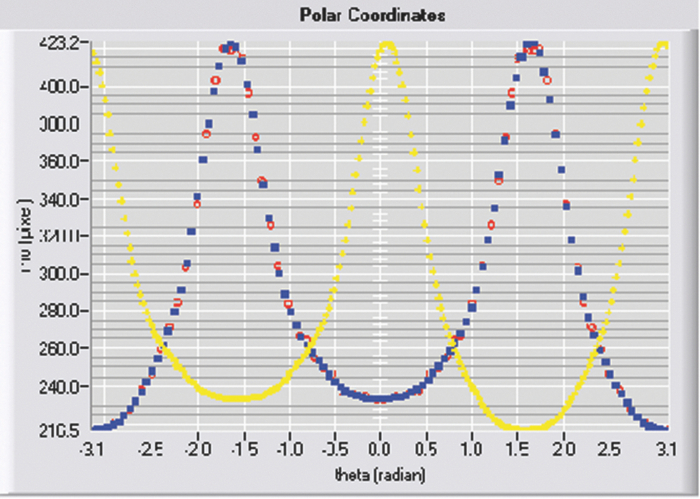
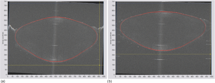
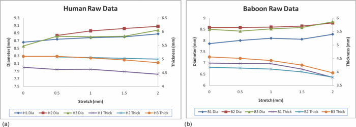
Typical OCT images of a baboon crystalline lens at different stages of accommodation using EVAS are shown in Figs. 1a and 1b. Fig. 1Raw OCT images of baboon crystalline lens; (a) Step 0–0 mm stretched; (b) Step 4–2 mm stretched. 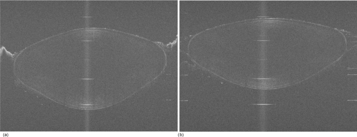 2.1.Edge DetectionEach lens images was manipulated with several image processing techniques to reliably extract and describe the outline of the lens. In the first step of the edge detection, the region of interest is selected manually to determine the general position of the lens within the image. This first step requires the user to move the two cursors on the image to the opposite corner of a rectangle, which outlines an ellipse around the lens shape that is enclosed by the rectangle. This selects the region of interest. All pixel values which lie outside the region of interest (generated ellipse) are discarded by setting the value of the pixels to zero. The “imaqSpoke” function from National Instruments IMAQ Vision “IMAQ_CVI.lib” library creates spokes which are represented by radial lines. These spokes are evenly spread at a fixed angle 4 deg about the center of the ellipse determined previously. In order to obtain a more even distribution of contour points, every second spokes line around the horizontal meridian which had a gradient less than a specific value representing the periphery, were omitted from the edge detection process. This gave a total number of 64 spoke lines. In the first step, the automated edge detection function was applied which searches and selects the first contour point with specified intensity value along each spoke from the outside toward the center. Obvious outliers and missing contour points can be corrected by manual user intervention. Instant graphical feedback is provided to assist the user with this process. 2.2.Lens ContourA pre-defined ellipse function from IMAQ_CVI.lib is fitted to the final set of the edge points to obtain a more accurate central reference point. This central reference point is used for transforming the edge data points into a polar coordinate system where each point is described by an angle (θ) and a radial distance (ρ). The two equatorial apex points are also obtained from the ellipse which was used to determine the angular misalignment of the lens. The image and detected edge points are rotated mathematically to correct for this tilt error. Based on the presumption that crystalline lenses are generally rotationally symmetric, the left right symmetry of the lens contour about the optical axis is then enforced by flipping left side points to right side about the center of the lens and then averaging the corresponding overlaid points. 2.3.Fourier Cosine SeriesAs described previously,22 a high order Fourier series can be fitted with the polar coordinates to obtain a mathematical description of the edge contour, which obeys constraints of continuity as well as zero to infinite surface slopes from apex to equator. The Fourier cosine series is described with the equation: Eq. 1[TeX:] \documentclass[12pt]{minimal}\begin{document}\begin{equation} \rho (\theta) = \sum\limits_{j = 0}^n {Aj \cdot \cos [j \cdot (\theta + } \alpha)], \end{equation}\end{document}Fitting high order Fourier cosine series to the detected points allowed interpolating of data points for small increments of angle θ (0.1 deg) by using the returned coefficients so that once converted back to the x-y pixel coordinate system, there would be a point for each pixel increment along the x-axis. The Fourier cosine series is fitted to the contour with the order that achieves the best fits. An algorithm was developed which determines this order number by means of comparing the mean square error (mse) value from the curve fit. Starting from the 14th order, it decrements until the mse value exceeds a specific percentage of the mse value at the 14th order. This process is automated initially, but user intervention is also implemented. Whenever the order number is changed, it plots the curve for the user to visualize the effect of different order of the Fourier cosine series. The last order number iteration is saved for future analysis. The Fourier cosine series enforces symmetry about the equatorial axis. Rotating the image and the detected edge points of the lens by 90° anticlockwise, forces the lens to be left right symmetry after being fitted with the Fourier cosine series. Once the Fourier cosine series is fitted, the image and Fourier cosine series points were rotated clockwise 90 deg. 2.4.Physical Lens ShapeThe physical shape of the lens was obtained by converting the pixel points of the OCT image to a millimeter scale by multiplying each pixel point by the image pixel resolution in the axial and lateral directions. For axial pixel to millimeter convertion, the scale factor included the refractive index of DMEM to convert optical to physical thickness. The lens thickness was measured by the minimum and the maximum coordinate in the direction of the optical axis. The lens diameter was measured by the minimum and the maximum coordinate in the direction of the equatorial axis. 2.5.Lens Surface CurvatureTo investigate how suitable and useful the Fourier cosine function is for the lens contour description and the curvature fitting of the central anterior and posterior pole region, other mathematical curve fitting functions to describe the shape of the lens based on the detected edge points were implemented and compared. While the Fourier cosine curves were fitted to the entire edge data point sets, separate curves were fitted for the anterior and posterior halves for the elliptical and polynomial curve fits. Mean square errors were calculated for each of the fitted curves as the average distance between the detected edge points and the intersection point on the fitted curve along corresponding radial lines. With the four sets of edge points (Fourier cosine, polynomial, best ellipse, and raw), radius of curvature and the eccentricity of the lens shape were calculated by fitting best ellipse and best circle curves along central 5 mm zones of the anterior and posterior profiles respectively. The best ellipse and circle fits are pre-defined functions available from National Instruments’ IMAQ Vision IMAQ_CVI.lib library. 2.6.Measurement RepeatabilityMeasurement repeatability was determined by analyzing one set of human data five times by the same user. The set of data consists of five images, captured at different steps of the stretch cycle. Diameter and thickness parameters were extracted and the standard deviations were determined. Based on this repeatability data, statistical significance can be determined for the changes in lens diameter and thickness between the stretching steps. 3.ResultsThe following results represent data for three sets of baboon and three sets of human lens at five different steps of the stretching with the EVAS instrument. All 30 OCT images were processed by the same operator, using the semiautomated process of determining the lens contour and shape as described above. Full and detailed results are presented for two typical set of data from one human and one baboon eye. Key numerical parameters are summarized for all eyes to illustrate variability and shape changes with lens stretching. Angular tilt of lens images was generally very small, ranging from 0.5 deg to a maximum of 8.0 deg. 3.1.Edge DetectionThe manual detection process facilitates the selection of points, which correspond closest to the edge contour of the lens. Figure 2 shows an ellipse which is determined by the two cursors enclosing the lens. Raw edge points are selected manually along each spoke and the obtained data set stored for further processing. Fig. 2Snapshot of the edge detection process, red spokes indicates periphery and blue spokes indicates central of the lens. Each spokes contains edge points. Cyan spoke shows the currently selected spoke and cyan point shows currently manually selected edge points along the spoke. All the points before the currently selected cyan spoke are manually selected by the user and points after the currently selected cyan spoke have not been manually selected yet showing points from automated edge detection process (rotating in anticlockwise direction).  3.2.Lens ContourAfter detecting all the lens edge points along the spoke, they were converted into polar coordinates as shown in Fig. 3. 3.3.Fourier Cosine SeriesThe polar coordinate is fitted with the Fourier cosine curve and is converted back to the x-y pixel point coordinate form. Now the contour of the crystalline lens is described as a mathematical description of the Fourier cosine series. An example of a Fourier cosine curve overlaying on the rotated image of the lens is shown in Figs. 4, 5. Note the different lateral scan width between the human lens (20 mm) and the baboon lens (10 mm). 3.4.Physical Lens ShapeFrom the raw data there was a trend of increase in the lens diameter and decrease in the lens thickness while the lenses were stretched. The trend was more obvious in baboon lenses compared to the human lenses, Fig. 6. After fitting Fourier cosine, polynomial, and elliptical functions to the raw data points, thickness, and diameter values were obtained again from each of the curve methods. Little variation was found between raw, cosine, and polynomial thickness, but the elliptical curve fit gave consistenly lower thickness values as shown in Fig. 7. This difference was statistically significant for all the baboon lenses at all steps, but less than half for the human lenses. 3.5.Lens Surface CurvatureDifferent curvatures were obtained from the manual detected points of the OCT images along the anterior and posterior surfaces by fitting Fourier cosine curve, polynomial curve, and the ellipse curve across the entire diameter of the lens. A typical example of the OCT image with different curvatures plotted is shown in Figs. 8, 9. Fig. 8Different curve fitting functions on the image. Yellow points are polynomial; green points are ellipse points along the purple ellipse curve fit; red points are cosine points; black points are manual detected points.[H1 lens Step 0 (a) and Step 4 (b)].  Fig. 9Different curve fitting functions on the image. Green points are ellipse points along the purple ellipse curve fit; Red points are cosine points; Yellow points are polynomial; Black points are manual points. [B3 lens Step 0 (a) and Step4 (b)].  Figures 10, 11 outline each curve fitting functions on separate images for the lens shown in Fig. 8 of Step 0 and Step 4, respectively. Fig. 10Different curve fitting functions outlined on separate images. Green points (a) are ellipse points along the purple ellipse curve fit; red points (b) are cosine points; yellow points (c) are polynomial; black points (d) are manual points. (H1 lens Step 0).  Fig. 11Different curve fitting functions outlined on separate images. Green points (a) are ellipse points along the purple ellipse curve fit; red points (b) are cosine points; yellow points (c) are polynomial; black points (d) are manual points. (H1 lens Step 4).  The error curve values were calculated separately for the anterior and posterior surfaces and are shown in Fig. 12a for human and Fig. 12b for baboon. All the points across the full diameter range of the lens were used in the calculation. The order for the Fourier cosine and polynomial curves was limited to 14 to avoid high frequency surface ripple effects. For both species, the elliptical fit improves as the lens is stretched. For the baboon lenses, the residual curve fit error for the ellipse was around twice as large compared to the Fourier cosine and polynomial curves. Using data points of each curve function obtained, best ellipse and best circle was fitted across 5 mm diameter from the center of the lens, to determine the radius of curvature and the eccentricity value for the anterior and posterior lens contour. Radius of curvature values are shown in Fig. 13a for one human and Fig. 13b for one baboon sample lens. Average results from three human lenses and three baboon lenses of the best circle and ellipse fits are summarized in Tables 2, 3, respectively. Fig. 13Radius of curvatures for both anterior and posterior surfaces for one human H1 (a) and one baboon B1 (b) lenses using best ellipse fitting across four different curve methods. 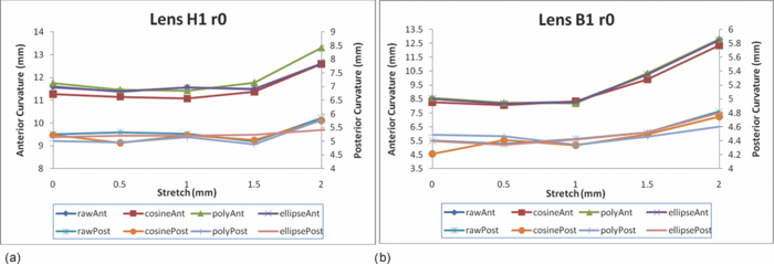 Table 3Averaged calculation of the radius (r) obtained from best circle, central radius thickness (r0) and eccentricity value (p) obtained from best ellipse fit on the four different curve functions for the three baboon lenses, unstretched and fully stretched.
Table 2Averaged calculation of the radius (r) obtained from best circle, central radius thickness (r0), and eccentricity value (p) obtained from best ellipse fit on the four different curve functions for the three human lenses, unstretched and fully stretched.
3.6.RepeatabilityFrom one randomly selected stretch cycle, each of the five images were analyzed by the same operator five times to obtain diameter and thickness values. A T-test was applied to determine if there was a statistically significant change in diameter or thickness between the unstretched and any of the Step 1 to Step 4 stretched images. Results and statistical significances are shown in Figs. 14a and 14b. The average standard deviation for repeated measurement was 0.04 mm for diameter and 0.02 mm for thickness. Variability between different operators may be slightly larger because of the inconsistency of subjective decision of detecting edges of the lens. The comparison of the diameter and thickness values at different steps was statistically insignificant for those without (*) mark compared to the values at 0 mm stretch. 4.DiscussionThe variable and low signal to noise ratio of OCT images had been a challenge for automated edge detection algorithms. Outliers and missing data points can lead to incorrect lens parameter extraction in subsequent processing steps. The semimanual edge detection method described in this study eliminates this problem by providing instant graphical feedback to the operator on selected raw data points as they are displayed and overlaid on the OCT image. Although this process is initially more time consuming, the subsequent processing steps become more reliable and require less error checking. The consistency of this process was verified and is sufficient to detect small changes in lens thickness and diameter associated with lens stretching. In this current study, we generated radial spokes across the entire lens emitting each line from the center of the lens for detecting edges. Chien et al,19 also used radial spokes, generating radial lines emitting from the origin starting at pole of anterior surface to the pole of posterior surface equally spaced at 2 deg. Most of the studies have described the lens profile separately for anterior and posterior surfaces using different functions. However Kasprak,20 using a hyperbolic cosine function modulated by hyperbolic tangent functions, mathematically described the lens as a single profile. Chien et al19 used a cosine function to fit the lens profile, however applied the function separately giving two sets of coefficients for anterior and posterior surfaces. As shown in this study, higher order Fourier cosine curve is suitable to describe the outline of crystalline lenses of different species and accommodation states as a single continuous profile. The order number for fitting Fourier cosine series is determined by the mse value. This iteration process was implemented to optimize the curve fitting function as different orders may be required to fit different type of species as well as for different stages of the stretch. Higher order Fourier cosine series generally provide a closer fit to the lens contour, but also introduce small ripples which compromise their application for further optical analysis, including ray tracing and analysis of higher order aberrations. To measure how well each curvature fitted to the manually detected points, the radial mean square errors between the fitted curve and the manually detected points was calculated. In general, as exemplified in Fig. 12, for accommodated and un-accommodated lenses, the ellipse fit showed the highest error for baboon lenses. This poor curve fitting is also reflected in the extracted lens thickness values whereby the thickness data obtained from the fitted elliptical curves was significantly less compared to other curve fittings. For human lenses, the ellipse fit showed similar error values compared to other curve fits for all different steps, which implies human lens’ are more elliptical in shape than the baboon lens. Fig. 12Error values calculated for each curve function across the full lens diameter for one human H1 (a) and one baboon B1(b) lenses. Anterior and posterior surfaces were calculated separately. 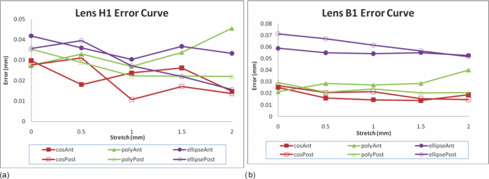 The posterior lens surface in all the images in this study are not corrected for the difference in refractive index between crystalline lens and DMEM, hence the results may vary from other studies which have been corrected22, 26 or do not suffer from optical distortions such as MRI4 or shadow photogrammetry.6 Our results for the human lens diameter and the thickness measurements obtained from the four different curve functions (Fourier cosine, polynomial, ellipse, and raw) is in broad agreement with previous studies by Pierscionek and Augusteyn,27 Jones et al,8 Rosen et al,6 and Urs 21 The thickness value for baboon (B1) lens was 4.32 mm which was slightly higher compared to other studies which was around 3.75 mm using phakometry Purkinje imaging technique of two 9 year old rhesus monkeys28 and slit-lamp Scheimpflug photography of rhesus monkeys.29 As the lenses were stretched, there was a trend of increase in lens diameter and decrease in lens thickness. This supports the Helmholtz theory of accommodation. Also, there was an increase in the radius of curvature values for anterior and posterior surfaces in both in human and baboon lenses, although least noticeable for the 65 years old human lens (H2). The anterior surface showed a steeper increase than the posterior surface in both the human and baboon species. This contradicts Chien et al30 who showed a decrease in the radius of curvature values as the lenses were stretched, but agrees well with most other authors.5, 28, 31 The radius of curvature value at the unaccommodated state for human lenses had been reported by various studies.2, 4, 5, 16 These results for the anterior and posterior radius of curvatures are very similar to our measurements. Using the ellipse fit, the average value of radii of curvatures across the four different curve fit method at the unaccommodated human lenses was 10.17±1.55 and 5.19±0.01 mm for anterior and posterior, respectively. Rosen et al6 reported slightly lower anterior radius of curvature 7.54±2.34 mm but similar posterior radius of curvature 5.5±0.9 mm. Schachar,32 however, reported higher posterior radius of curvature of 7.1±1.0 mm. The differences may be explained by the varying central diameter range selected which Schachar used to fit the elliptical curves. The raw data average radius of curvatures for three baboon lenses was 8.84±0.68 mm for anterior surface was and 5.49±1.27 mm for the posterior surface at the un-accommodated state. This value was lower compared to the study Rosales 28 performed, which was 11.11±1.58 and 6.64±0.62 mm for anterior and posterior, respectively. The study performed by Rosales used rhesus monkeys which had undergone removal of the iris and implantation of stimulating electrodes into the EW nucleus. These may contribute in the difference in the results performed in our current study. 5.ConclusionIn this study, modified methods and algorithms were presented to obtain more accurate contours from crystalline lens OCT images compared to previous attempts.22 The process of semimanual detection of edge points along the contour of the lens provides reliable raw data points for further mathematical description and analysis. Describing the lens contour with a single continuous profile by fitting a Fourier cosine series is a valid method for various shapes and species of lenses and is useful to investigate the changes in lens shape with age and accommodation to better understand the condition of presbyopia. The measured flattening of the central anterior and posterior human and baboon lens profiles as the lens is stretched, supports the Helmholtz theory of accommodation. Analyzing different species (human and baboon) at different stages of the stretch also emphasize the ability for the outlined algorithms to work for different types and shapes of the lenses. This analysis and description of the lens shape can be used to further characterize the optical properties of the lens, in particular optical power, aberrations, and gradient refractive index. AcknowledgmentsWe gratefully acknowledge the tissue donated by the Florida Lions and other U.S. Eye Banks and the University of Miami Diabetic Research Institute and Division of Veterinary Resources. The research was supported in part by Vision CRC Sydney Australia; NIH-NEI 2R01EY14225 (KE, JMP); NIH center Grant No. P30-EY014801 and NIH Ruth L. Kirschstein NRSA F32 EY15630 (SRU); the Florida Lions Eye Bank, Research to Prevent Blindness, and the Henri and Flore Lesieur Foundation (JMP). ReferencesA. Glasser and
M. C. Campbell,
“Presbyopia and the optical changes in the human crystalline lens with age,”
Vision Res., 38
(2), 209
–229
(1998). https://doi.org/10.1016/S0042-6989(97)00102-8 Google Scholar
P. Rosales, M. Dubbelman, S. Marcos, and
R. Van Der Heijde,
“Crystalline lens radii of curvature from Purkinje and Scheimpflug imaging,”
J. Vision, 6
(10), 1057
–1067
(2006). https://doi.org/10.1167/6.10.5 Google Scholar
L. F. Garner,
“Calculation of the radii of curvature of the crystalline lens surfaces,”
Ophthalmic Physiol. Opt., 17
(1), 75
–80
(1997). https://doi.org/10.1111/j.1475-1313.1997.tb00527.x Google Scholar
J. F. Koretz, S. A. Strenk, L. M. Strenk, and
J. L. Semmlow,
“Scheimpflug and high-resolution magnetic resonance imaging of the anterior segment: a comparative study,”
J. Opt. Soc. Am. A, 21
(3), 346
–354
(2004). https://doi.org/10.1364/JOSAA.21.000346 Google Scholar
E. A. Hermans, P. J. Pouwels, M. Dubbelman, J. P. Kuijer, G. L. Van Der Heijde, and
R. M. Heethaar,
“Constant volume of the human lens and decrease in surface area of the capsular bag during accommodation: An MRI and Scheimpflug study,”
Invest Ophthalmol. Vis. Sci., 50
(1), 281
–289
(2009). https://doi.org/10.1167/iovs.08-2124 Google Scholar
A. M. Rosen, D. B. Denham, V. Fernandez, D. Borja, A. Ho, F. Manns, J. M. Parel, and
R. C. Augusteyn,
“In vitro dimensions and curvatures of human lenses,”
Vision Res., 46
(6–7), 1002
–1009
(2006). https://doi.org/10.1016/j.visres.2005.10.019 Google Scholar
L. F. Garner and
M. K. Yap,
“Changes in ocular dimensions and refraction with accommodation,”
Ophthalmic Physiol. Opt., 17
(1), 12
–17
(1997). https://doi.org/10.1111/j.1475-1313.1997.tb00518.x Google Scholar
C. E. Jones, D. A. Atchison, R. Meder, and
J. M. Pope,
“Refractive index distribution and optical properties of the isolated human lens measured using magnetic resonance imaging (MRI),”
Vision Res., 45
(18), 2352
–2366
(2005). https://doi.org/10.1016/j.visres.2005.03.008 Google Scholar
D. Huang, E. A. Swanson, C. P. Lin, J. S. Schuman, W. G. Stinson, W. Chang, M. R. Hee, T. Flotte, K. Gregory, C. A. Puliafito, and
J. G. Fujimoto,
“Optical coherence tomography,”
Science, 254 1178
–1181
(1991). https://doi.org/10.1126/science.1957169 Google Scholar
M. Gora, K. Karnowski, M. Szkulmowski, B. J. Kaluzny, R. Huber, A. Kowalczyk, and
M. Wojtkowski,
“Ultra high-speed swept source OCT imaging of the anterior segment of human eye at 200 kHz with adjustable imaging range,”
Opt. Express, 17
(17), 14880
–14894
(2009). https://doi.org/10.1364/OE.17.014880 Google Scholar
I. Grulkowski, M. Gora, M. Szkulmowski, I. Gorczynska, D. Szlag, S. Marcos, A. Kowalczyk, and
M. Wojtkowski,
“Anterior segment imaging with spectral OCT system using a high-speed CMOS camera,”
Opt. Express, 17
(6), 4842
–4858
(2009). https://doi.org/10.1364/OE.17.004842 Google Scholar
S. R. Uhlhorn, D. Borja, F. Manns, and
J. M. Parel,
“Refractive index measurement of the isolated crystalline lens using optical coherence tomography,”
Vision Res., 48
(27), 2732
–2738
(2008). https://doi.org/10.1016/j.visres.2008.09.010 Google Scholar
M. C. M. Dunne, L. N. Davies, and
J. S. Wolffsohn,
“Accuracy of cornea and lens biometry using anterior segment optical coherence tomography,”
J. Biomed. Opt., 12
(6), 064023
(2007). https://doi.org/10.1117/1.2821844 Google Scholar
A. Glasser and
M. C. Campbell,
“Biometric, optical and physical changes in the isolated human crystalline lens with age in relation to presbyopia,”
Vision Res., 39
(11), 1991
–2015
(1999). https://doi.org/10.1016/S0042-6989(98)00283-1 Google Scholar
D. Borja, F. Manns, A. Ho, N. Ziebarth, A. M. Rosen, R. Jain, A. Amelinckx, E. Arrieta, R. C. Augusteyn, and
J. M. Parel,
“Optical power of the isolated human crystalline lens,”
Invest Ophthalmol. Vis. Sci., 49
(6), 2541
–2548
(2008). https://doi.org/10.1167/iovs.07-1385 Google Scholar
M. Dubbelman and
G. L. Van Der Heijde,
“The shape of the aging human lens: curvature, equivalent refractive index and the lens paradox,”
Vision Res., 41
(14), 1867
–1877
(2001). https://doi.org/10.1016/S0042-6989(01)00057-8 Google Scholar
R. Urs, F. Manns, A. Ho, D. Borja, A. Amelinckx, J. Smith, R. Jain, R. Augusteyn, and
J. M. Parel,
“Shape of the isolated ex-vivo human crystalline lens,”
Vision Res., 49
(1), 74
–83
(2009). https://doi.org/10.1016/j.visres.2008.09.028 Google Scholar
R. A. Schachar, T. Huang, and
X. Huang,
“Mathematic proof of Schachar's hypothesis of accommodation,”
Ann. Ophthalmol., 25
(1), 5
–9
(1993). Google Scholar
C. H. Chien, T. Huang, and
R. A. Schachar,
“A mathematical expression for the human crystalline lens,”
Compr. Ther., 29
(4), 245
–258
(2003). https://doi.org/10.1007/s12019-003-0028-1 Google Scholar
H. T. Kasprzak,
“New approximation for the whole profile of the human crystalline lens,”
Ophthalmic Physiol. Opt., 20
(1), 31
–43
(2000). https://doi.org/10.1016/S0275-5408(99)00031-9 Google Scholar
R. Urs, A. Ho, F. Manns, and
J.-M. Parel,
“Age-dependent Fourier model of the shape of the isolated ex vivo human crystalline lens,”
Vision Res., 50
(11), 1041
–1047
(2009). https://doi.org/10.1016/j.visres.2010.03.012 Google Scholar
E. Kim, K. Ehrmann, S. Uhlhorn, D. Borja, and
J.-M. Parel,
“Automated analysis of OCT images of the crystalline lens,”
Proc. SPIE, 7163 716313
(2009). https://doi.org/10.1117/12.809986 Google Scholar
K. Ehrmann, A. Ho, and
J.-M. Parel,
“Ex vivo accommodation simulator II: concept and preliminary results,”
Proc. SPIE, 5314 48
(2004). https://doi.org/10.1117/12.539111 Google Scholar
K. Ehrmann, A. Ho, and
J.-M. Parel,
“Evaluation of porcine crystalline lenses in comparison with molded polymer gel lenses with an improved ex vivo accommodation simulator,”
Proc. SPIE, 5688 240
–251
(2005). https://doi.org/10.1117/12.599223 Google Scholar
K. Ehrmann, A. Ho, and
J.-M. Parel,
“Biomechanical analysis of the accommodative apparatus in primates,”
Clin. Exp. Optom., 91
(3), 302
–312
(2008). https://doi.org/10.1111/j.1444-0938.2008.00247.x Google Scholar
D. Borja, D. Siedlecki, A. de Castro, S. Uhlhorn, S. Ortiz, E. Arrieta, J. M. Parel, S. Marcos, and
F. Manns,
“Distortions of the posterior surface in optical coherence tomography images of the isolated crystalline lens: effect of the lens index gradient,”
Biomed. Opt. Express, 1
(5), 1331
–1339
(2010). https://doi.org/10.1364/BOE.1.001331 Google Scholar
B. K. Pierscionek and
R. Augusteyn,
“Shapes and dimensions of in vitro human lenses,”
Clin. Exp. Optom., 74
(6), 223
–228
(1991). https://doi.org/10.1111/j.1444-0938.1991.tb04646.x Google Scholar
P. Rosales, M. Wendt, S. Marcos, and
A. Glasser,
“Changes in crystalline lens radii of curvature and lens tilt and decentration during dynamic accommodation in rhesus monkeys,”
J. Vision, 8
(1), 1
–12
(2008). https://doi.org/10.1167/8.1.18 Google Scholar
J. F. Koretz, A. Bertasso, M. Neider, B. a. True-Gabelt, and
P. Kaufman,
“Slitp-lamp studies of the Rhesus Monkey Eye: Changes in crystalline lens shape, thickness, and position during accommodation and aging,”
Exp. Eye Res., 45 317
–326
(1987). https://doi.org/10.1016/S0014-4835(87)80153-7 Google Scholar
C. H. Chien, T. Huang, and
R. A. Schachar,
“Analysis of human crystalline lens accommodation,”
J. Biomec., 39
(4), 672
–680
(2006). https://doi.org/10.1016/j.jbiomech.2005.01.017 Google Scholar
M. Dubbelman, G. L. Van Der Heijde, and
H. A. Weeber,
“Change in shape of the aging human crystalline lens with accommodation,”
Vision Res., 45
(1), 117
–132
(2005). https://doi.org/10.1016/j.visres.2004.07.032 Google Scholar
R. A. Schachar,
“Central surface curvatures of postmortem- extracted intact human crystalline lenses: implications for understanding the mechanism of accommodation,”
J. Ophthalmol., 111
(9), 1699
–1704
(2004). https://doi.org/10.1016/S0161-6420(04)00669-4 Google Scholar
|
|||||||||||||||||||||||||||||||||||||||||||||||||||||||||||||||||||||||||||||||||||||||||||||||||||||||||||||||||||||||||||||||||||||||||||||||||||||||||||||||||||||||||||||||||||||||||||||