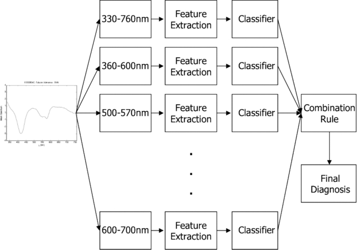
1.1.

Spectral Classification for Diagnostic Spectroscopy

The promise of optically guided biopsy using elastic-scattering spectroscopy (ESS) in colorectal cancer screening relies on achieving a high accuracy for detecting neoplasms, because misdiagnoses can be potentially costly. Both statistical and model-based methods of spectral classification have been studied by a number of groups.^{1, 2, 3, 4}

The present report focuses on improvements in pattern-recognition and machine-learning methods, as applied to ESS, with the complexities of biological variability in mind. The specific clinical application addressed here is the assessment of polyps during colonoscopy for the screening/management of colorectal cancer.

Current algorithms, based on a single classifier, have shown the feasibility of ESS as a diagnostic tool,^{1, 2, 5, 6, 7} yet increased accuracy is desired for ESS to be widely adopted in clinical settings, particularly for the in situ classification of polyps during colorectal cancer screening.⁸ A different classifier framework, one where the decision is made based on the input from various classifiers, can enhance performance over a single-classifier scheme.^{9, 10, 11, 12} This field of combining multiple classifiers, or ensemble classifiers, has garnered increased attention over the past decade in the pattern-recognition and machine-learning community motivated by the prospect of improving classification performance. Ensemble classifiers are generally designed based on different approaches for generating the base classifiers (i.e., the set of classifiers that composes the ensemble).¹¹ One approach, the data level, uses different subsets of the training data to design the base classifiers. Two common sampling methods to achieve this include bagging and boosting,^{11, 13} with AdaBoost^{11, 14, 15} being a well-known classifier employing the latter method. In a second approach, the feature level, the base classifiers are designed on different subsets of data features. This approach was used to classify autofluorescence spectra acquired from healthy and diseased mucosa in the oral cavity.¹⁰ Another approach is the classifier level, where each of the base classifiers is designed using a different classification method. Tumer ¹² employed the classifier-level approach when classifying fluorescence spectra for cervical dysplasia by designing ensembles with different radial basis-function neural networks as base classifiers.

An additional classification paradigm can also be used to improve current performance levels. The misclassification-rejection (MR) approach, known in the literature as error-rejection, is one where the classifier identifies samples at high risk of being misclassified, in most cases the ones lying near the decision boundary, and as such, refrains from making a decision on them. Thus, for a binary classification problem there is a third possible outcome: A sample is not assigned a class or label, and is considered as a rejected sample. The expected result is an improvement in performance relative to the one obtained with a regular classifier at the expense of having a percentage of the samples not classified. Rejected samples would then have to be examined by some other method (repeat optical measurements or biopsy) in order to obtain their classification. With this paradigm, decisions become a sequential process, suitable for colonoscopic cancer screening, where an initial real-time, in vivo examination of a polyp using ESS is followed by biopsy and histopathology if it could not be classified spectroscopically.

The idea of misclassification-rejection has been mentioned for spectroscopic applications;^{16, 17} however, no formal framework has been presented. The concept of misclassification-rejection was first introduced by Chow¹⁸ for minimum probability of error classifiers, where the optimal decision rules take the form of a threshold for the posterior probabilities, assuming that the underlying probability distributions are known. Extensions to this work have been presented for cases where the underlying probability distributions are unknown and estimated;^{19, 20} artificial neural networks;^{21, 22} and support vector machines (SVM).^{23, 24, 25, 26, 27} In addition, reformulations of the SVM training problem, embedding the rejection option have been presented.^{28, 29, 30} In this framework, the decision boundary becomes a decision region that, in its simplest form, consists of a pair of parallel hyperplanes separated by some distance. Samples lying within this decision region are rejected. In this paradigm, the orientation of the decision regions as well as the distance between them are obtained during the training phase, in contrast to previous work that has focused on methods to threshold samples once the classifier has been designed. This has resulted in an improvement in error-reject trade-off when compared to simply thresholding the output after designing the classifier. The notion of misclassification-rejection for classifying spectra in “optical biopsy” schemes can be thought of as relating to the all-too-frequent histopathology designation of “indeterminate,” or to cases where multiple histopathology assessments of the same tissue lack agreement. A different type of “error” identification has been introduced by Zhu,³¹ wherein principal components that relate to variations in practitioner technique (e.g., probe pressure, angle) are ignored in the classification. These differences are often variations of overall intensity, and their removal can lead to improvement in classification performance.^{31, 32} Another type of error rejection is often referred to as “outlier rejection,” in which spectra that clearly invoked experimental error (e.g., broken probe, noncontact with the tissue, or dirt on the probe tip) are rejected. Both of these error types differ from our misclassification-risk reduction, which is more akin to identifying biological uncertainly. In our experimental approach, such outliers can be recognized and instantly rejected at the moment of the measurement.

1.2.

Optical Biopsy in Management of Colorectal Cancer

In the United States, colorectal cancer (CRC) is the second leading cause of cancer and cancer death for both sexes (behind lung cancer), with nearly 150,000 new cases and 50,000 deaths annually in recent years.³³ Current recommendations from multiple professional societies advocate early detection by screening the entire average-risk population for CRC beginning at age 50.³⁴ Accepted screening modalities include (i) stool occult blood or deoxyribose nucleic acid testing, (ii) flexible sigmoidoscopy every five years (iii) colonoscopy every 10 years, and (iv) radiological examination via double-contrast barium enema or computed tomography colonography every five years. Of these, colonoscopy emerged as the most effective method of screening because a high-quality examination permits simultaneous detection and removal of precancerous polyps, thus modifying CRC risk.³⁵

The effectiveness of colonoscopic cancer prevention hinges on the complete removal of all polyps detected during a standard-definition white-light endoscopy (SDWLE).^{35, 36, 37} However, a large proportion (up to 50%) of polyps that are removed are, in fact, non-neoplastic by histopathology (i.e., they have negligible malignant potential). Thus, there is an inherent inefficiency: Because neoplastic and non-neoplastic polyps cannot be reliably distinguished by SDWLE alone, substantial resources are devoted to the removal of clinically inconsequential tissue, while the actual benefit derives from the identification and removal of premalignant lesions. Thus, there is great need for simple, rapid, and low-cost methods for “smart” tissue evaluation, because removing inconsequential tissue introduces additional unnecessary time, cost, and incremental risk of bleeding and perforation, to a high-demand, high-volume screening procedure.

Optical spectroscopy has been suggested to assist endoscopists in classifying polyps in situ and in real time in a simple and cost-effective manner.^{1, 2, 3, 4} In particular, ESS has shown promise for detecting dysplasia and/or cancer in various epithelial-lined hollow organs, including the urinary bladder,³⁸ esophagus,^{7, 39, 40, 41, 42} and colon,^{1, 2, 3} as well as in tissues such as breast and lymph nodes.^{5, 6} ESS, mediated by specific fiberoptic probes with specific optical geometries, is sensitive to the absorption spectra of major chromophores (e.g., oxy-/deoxy-hemoglobin) and, more importantly, the scattering spectra, which relate to micromorphological features of superficial tissue. ESS spectra derive from the wavelength-dependent optical scattering efficiency (and the effects of changes in the scattering angular probability) caused by optical index gradients exhibited by cellular and subcellular structures. Unlike Raman and fluorescence spectroscopy, ESS provides largely microstructural, not biochemical, information. ESS is sensitive to features such as nuclear size, crowding, and chromaticity, chromatin granularity, and mitochondrial and organellar size and density [Fig. 1a]. Because neoplasia is associated with changes in subcellular, nuclear, and organellar features, scattering signatures represent the spectroscopic equivalent of a histopathological interpretation. The ESS method, however, senses morphological changes semiquantitatively without actually rendering a microscopic image.^{43, 44} In practice, ESS is a point-source measurement obtained over a broad wavelength range (320–900 nm) that samples a tissue volume of ≤0.1 mm³. Probes are comprised of separate illuminating and collecting fibers [Fig. 1b] and require optical contact with tissue being interrogated. Collected light transmitted to the analyzing spectrometer must first undergo one or more scattering events through a small volume of the tissue before entering the collection fiber(s) in the “backward” direction. No light is collected from surface Fresnel reflection. The standard ESS catheter-type probe consists of a pair of fibers (each with a core diameter of 200 μm) with a center-to-center separation of ∼250 μm. Because of the small separation of the source and detector fibers, the collected light predominantly samples the mucosal layer, which is typically 300–400 μm thick in the GI tract.

Fig. 1

(a) Cartoon illustration of optical scattering from density gradients in cells, and (b) a diagram of the optical geometry for the fiber-optic tissue measurements. Fiber tips are in optical contact with the tissue surface. Only light that has scattered elastically within the epithelial layer is collected.

Ideally, when using elastic-scattering spectroscopy, some form of spectral analysis is performed on the collected measurements of the examined tissue. ESS was first applied in vivo in the urinary bladder by Mourant,³⁸ where correlation of spectral features, determined “by inspection,” for the detection of malignant tissue in a retrospective analysis from a small sample size (110 biopsy sites from 10 patients) showed the feasibility of ESS as a diagnostic tool. Bigio ⁵ used artificial neural networks (ANN) to classify ESS spectra from breast tissue and sentinel nodes. Analysis resulted in sensitivities of 69 and 58%, and specificities of 85 and 93%, for breast tissue and sentinel nodes, respectively. In another study by Ge,² light-scattering spectra of neoplastic and non-neoplastic colonic polyps could be distinguished using multiple linear regression analysis, linear discriminant analysis (LDA), and ANN. Sensitivities and specificities of 91% and 78%, 91% and 74%, and 79% and 91% were obtained, respectively, for each of the three methods. Dhar ¹ used LDA and leave-one-out cross-validation to classify several colonic lesions, among them adenomatous versus hyperplastic polyps, with a sensitivity of 84% and specificity of 84%, adenocarcinoma versus normal colonic mucosa, with a sensitivity of 80% and specificity of 86%, and adenocarcinoma versus adenomatous polyps, with a sensitivity of 80% and specificity of 75%. In addition to these statistical pattern-recognition approaches, model-based classifications have been proposed, primarily based on extracting nuclear size distribution from the scattering spectra. These have yielded performances comparable to statistical approaches.^{4, 45, 46} The advantages of using ensemble classifiers and misclassification-rejection, described here, are intended to provide diagnostic information of higher reliability, with the benefit of providing an assessment of the risk of misclassification. The resulting improved method is tested prospectively on a naïve data set.

2.1.

Instrumentation

The ESS system and integrated forceps have been previously described.⁴⁷ Briefly, when using ESS, or any point spectroscopic measurement, it is essential to coregister precisely the optical reading and the physical biopsy. With this in mind, an endoscopic tool that integrates an ESS probe with a biopsy forceps was designed. In order to incorporate an ESS probe into the biopsy forceps, it was necessary to reduce the diameter of the optical fibers. In previous studies, the illuminating fiber was a 400-μm core optical fiber and the backscatter detector a 200-μm fiber. For the integrated ESS optical biopsy forceps, two 200-μm core fibers (source and detector) were used, each with a numerical aperture of 0.22 in air. The center-to-center separation between the fibers was ∼250 μm. Biopsy forceps were built with a hollow central channel that extended to the space between the jaws (SpectraScience, San Diego, California) capable of accommodating the 0.470-mm diameter of the hypotube encasing the probe (Fig. 2).

Fig. 2

(a) Two-dimensional diagram of the forcep tip is depicted. The optical forcep is a modified traditional endoscopic jaw-type biopsy forcep (left) with a central channel through which fiberoptic probes can be introduced for tissue measurements (right). (b) A photograph of a clinically-usable unit, standard biopsy forceps (left), ESS integrated optical forceps (right).

Similar to previously described ESS designs, the forceps connect to the ESS system, which consists of a pulsed Xenon-arc lamp (LS-1130-3, Perkin Elmer, Waltham, Massachusetts) broadband light source, a built-in computer with custom ESS software, and built-in spectrometer (S2000, Ocean Optics, Inc., Dunedin, Florida), microcontroller board and power supplies (Fig. 3). Before each procedure, the ESS forceps and spectrometer were calibrated for system response by measuring the reflectance from a spatially flat diffuse-reflector Spectralon (Labsphere Inc., North Sutton, New Hampshire) to standardize for variations in the light source, spectrometer, fiber transmission, and fiber coupling. It should be noted that the endoscope light source (Olympus 100 series with Evis Exera I and II systems) does not interfere with ESS readings, because the background light is measured separately and subtracted from the ESS measurement.

Fig. 3

(a) Schematic diagram of the ESS system and (b) photo of portable ESS optical biopsy system.

2.2.

Clinical Measurements

Data collection was performed under an ongoing IRB-approved clinical study at the Veterans Affairs Medical Center, Boston, Massachusetts. Subjects were recruited from among individuals scheduled for a medically indicated screening or surveillance colonoscopy. When a polyp or suspicious growth was encountered by the endoscopist during the procedure, the forceps jaws were opened such that the central optical probe was placed in gentle contact with the identified polyp and five ESS measurements were taken in rapid succession. Once the optical readings were obtained, the forceps jaws were closed to obtain the physical biopsy. By using forceps with integrated ESS optics, precise coregistration of optical readings and physical biopsies is assured. Three specialist gastrointestinal pathologists, using predefined standard histopathological criteria, reviewed each endoscopic pinch biopsy independently. The “optical biopsies” were then correlated to the majority classification by histopathology.

2.3.

Data Processing and Analysis

2.3.4.

Ensemble classifiers

When developing an ensemble classifier for classification of ESS spectra, we intended to take advantage of the high dimensional nature of the data. For this purpose, a feature-level approach, as discussed earlier, is used. In this approach, the ensemble is created by designing each base classifier on a subset of the sample pattern's features. An important aspect of ensemble classifiers is diversity among the base classifiers (i.e., trying not to commit errors on the same samples).^{9, 11} With this in mind, we propose using the ensemble classifier architecture illustrated in Fig. 4. The system consists of a number of parallel classifiers, each trained on a region of the ESS spectrum. The design of each of the base classifiers involves a feature extraction (PCA) step followed by the training of a linear SVM classifier with those particular extracted features. Diversity is introduced by training the base classifiers on different subspaces generated by the extracted features.

Fig. 4

Proposed ensemble classifier architecture.

The final classification, or diagnosis, is obtained by combining the outputs of the base classifiers. Because we are working with SVM, whose output is a class label, combination rules that fuse label classifier outputs will be used. Two combination rules, majority-voting and naïve Bayes combiner, were considered. The majority-voting rule assigns a sample the class label that 50% + 1 or more of the base classifiers agree on. In the case of a tie when using even numbers of base classifiers, the member of the ensemble with the highest classification accuracy breaks the tie. The naïve Bayes combination rule is stated as follows:¹¹ let x be a sample vector belonging to one of the possible ω_k, k = 1, …, c classes. Also let L be the number of base classifiers in the ensemble. The ensemble classifies a sample x as belonging to class ω_k if σ_k(x) is maximum, where

Eq. 5

[TeX:] \documentclass[12pt]{minimal}\begin{document}\begin{equation} \sigma _k ({\bf x})\propto \,P\left({\omega _k } \right)\prod\limits_{i = 1}^L P \left({y_i |\omega _k } \right), \end{equation}\end{document} $${\sigma }_k\left(\mathbf{x}\right)\propto P\left({\omega }_k\right)\prod _{i=1}^{L}P\left(y_i|{\omega }_k\right),$$

and y _i is the output label from the i’th base classifier. For the practical application of the binary classification of non-neoplastic (ω_{non-neoplastic}) versus neoplastic (ω_neoplastic) tissue, and assuming that, if y _i = 1 the sample is classified as non-neoplastic, and if y _i = –1, the sample is classified as neoplastic by the base classifiers, the conditional probabilities can be estimated as

Eq. 6

[TeX:] \documentclass[12pt]{minimal}\begin{document}\begin{equation} \begin{array}{l} P\left({y_i = - 1|\omega _{neoplastic} } \right) = {\rm Sensitivity}, \\[5pt] P\left({y_i = 1|\omega _{neoplastic} } \right) = 1 - {\rm Sensitivity}, \\[5pt] P\left({y_i = 1|\omega _{non - neoplastic} } \right) = {\rm Sensitivity}, \\[5pt] P\left({y_i = - 1|\omega _{non - neoplastic} } \right) = 1 - {\rm Sensitivity}, \\[5pt] \end{array} \end{equation}\end{document} $$\begin{array}{c}P\left(y_i=-1|{\omega }_{neoplastic}\right)=\mathrm{Sensitivity},\hfill \\ P\left(y_i=1|{\omega }_{neoplastic}\right)=1-\mathrm{Sensitivity},\hfill \\ P\left(y_i=1|{\omega }_{non-neoplastic}\right)=\mathrm{Sensitivity},\hfill \\ P\left(y_i=-1|{\omega }_{non-neoplastic}\right)=1-\mathrm{Sensitivity},\hfill \end{array}$$

P(ω_k) are the prior probabilities and can be estimated from the training data. Thus, this combination rule uses the performance of each base classifier, in the form of the sensitivity and specificity, to weight their individual decision when making the final classification.

3.1.

Data Set

The data set consists of 494 elastic-scattering spectroscopy (ESS) measurements from 297 polyps from 134 patients. Because our work will concentrate on binary classifiers, the samples were grouped into two clinically relevant classes, non-neoplastic samples and neoplastic samples. Of the 297 polyps measured 199 correspond to non-neoplastic tissue including hyperplastic polyps, histologically normal growths, and inflammatory polyps, while 98 correspond to neoplastic polyps and adenocarcinomas. A total of 325 spectra were collected from the non-neoplastic sites and 169 from the neoplastic sites.

The data set was divided into separate training and testing sets for design and testing of the presented classifiers. Using the same training and testing sets will also permit the comparison and evaluation of the proposed classifiers in a standardized manner. The data was partitioned by randomly assigning 80 patients (60%) to the training set, from which 193 spectra from 111 non-neoplastic polyps and 92 spectra from 54 neoplastic polyps were acquired and the remaining 54 patients (40%) to the testing set, from which 132 spectra from 88 non-neoplastic polyps and 77 spectra from 44 neoplastic polyps were acquired. Table 1 summarizes the number of cases per pathology for the training and testing sets. Figure 5 illustrates the representative spectra for each class, as well as their standard deviation, for the training and testing set.

Fig. 5

Representative spectrum for each class: (a) training set and (b) testing set.

Fig. 8

Performance (sensitivity and specificity) as a function of rejection rate obtained using the error-rejection classification paradigm.

Table 1

Data-set breakdown.

3.2.

Spectral Classification

To establish a performance baseline for classifying neoplastic and non-neoplastic polyps using ESS, we used the standard classification paradigm of dimensionality reduction followed by classification, as this approach has been commonly used for spectral analysis. ^{1, 2, 5, 7, 16, 17, 52, 53, 54, 55, 56, 57} The training data was used to compute the transformation matrix V for PCA and to determine the number of PCs used to train the classifier, in this case an SVM with linear kernel. The number of PCs was determined by performing cross-validation on the training set while increasing the number of PCs used, and selecting the number after which no increase in performance was observed. SVM parameters were chosen from a finite set of values and by selecting those that showed the best performance on the training set. The full spectral range, 330–760 nm, was used and the first 15 principal components were used for classification. Results from the testing set reveal that this classification scheme can differentiate ESS spectra of neoplastic from spectra of non-neoplastic lesions with a sensitivity of 0.83 and specificity of 0.79 with an overall accuracy of 0.80. Figure 6 shows the averages and standard deviations of the reconstructed dataset, using Eq. 2, with the selected principal components. By using a single principal component, or a subset of components, to do this transformation, the reconstructed data will express the variance along those specific directions, revealing areas of the spectrum found to be informative by PCA. In Fig. 6b, it can be seen that the variance in the data is predominant at ∼330–600 nm when using the first PC. The variance is more contained around 330–380 nm, 410–440 nm, 480–625 nm, and 650–760 nm when using PC 2 to PC 15 [Fig. 6c]. In PC 3 to PC 15, we see that it is localized around 330–360 nm, 460–500 nm, and near 420 nm and 575 nm [Fig. 6d], with this trend remaining in subsequent PCs [Figs. 6e, 6f].

Fig. 6

(a)Training set representative spectrum for each class, (b) reconstructed data using the first PC, (c) reconstructed data using PC2 to PC15, (d) reconstructed data using PC3 to PC15, (e) reconstructed data using PC4 to PC15, and (f) reconstructed data using PC5 to PC15.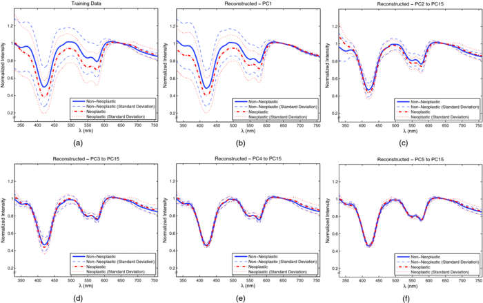

3.2.1.

Ensemble classifiers

To construct the ensemble classifier proposed in Sec. 2.3.4 (Fig. 4) a series of classifiers were trained on specific regions of the ESS spectrum, using the standard classification paradigm, with PCA used for feature extraction and a linear SVM for classification. This set, or subsets, of classifiers will be used as the base classifiers in our scheme. A total of 12 regions were chosen empirically, taking into consideration the observations from principal component analysis discussed earlier. Regions were selected based on the spectral areas that exhibited the largest variance when the data were reconstructed with specific PCs (Fig. 6). These spectral areas are considered the most informative based on the PCA criterion. In addition, we made sure that spectral regions containing the hemoglobin Soret (∼400–440 nm) and Q (∼540–580 nm) bands were included, as well as the ranges of ∼330–370 nm and ∼380–500 nm since these have been found to be informative for distinguishing pathologies.^{3, 38} Table 2 summarizes the performance of the individual base classifiers. The best performance, accuracy of 0.80 was obtained using the full spectrum (i.e., 330–760 nm). The worst performance, accuracy of 0.67, was obtained in the region of 600–700 nm. Regions in the shorter wavelengths (<460 nm) exhibited better overall performance, with the performance of 330–400 nm, Se = 0.84, Sp = 0.73, on par with the performance when using the entire spectrum, Se = 0.83, Sp = 0.79. Table 3 shows, for each pair of regions, the fraction of the total misclassifications where both regions misclassified the same sample. It is desirable for this metric to have a small value as ideally the base classifiers in the ensemble commit errors on different samples, allowing for correction of these errors as the ensemble is taken as a whole. Although the regions were not completely independent and uncorrelated, because some overlap among them was allowed, it is observed that the resulting classifiers are committing errors on different samples. Even between regions with significant overlap (e.g., 330–760 nm and 330–600 nm, 360–460 nm, and 360–600 nm, 500–530 nm, and 500–570 nm), the fraction of total misclassifications where both regions misclassified the same sample was, at worst, around 0.70 (Table 3). This outcome is meaningful in the context of ensemble classifiers because this means that diversity is being promoted by this approach, including cases when regions overlap.

Table 2

Performance of classifiers trained on each region.

Index	Region (nm)	PCs	Sensitivity	Specificity	Accuracy
1	330–760	15	0.83	0.79	0.80
2	330–600	15	0.82	0.76	0.78
3	360–600	14	0.83	0.74	0.78
4	360–460	14	0.87	0.69	0.76
5	500–570	5	0.71	0.77	0.75
6	500–530	3	0.73	0.70	0.71
7	540–570	3	0.73	0.72	0.72
8	360–400	4	0.87	0.59	0.69
9	330–360	7	0.79	0.71	0.74
10	600–700	20	0.66	0.68	0.67
11	330–400	8	0.84	0.73	0.78
12	380–460	11	0.70	0.77	0.75

Table 3

Fraction of total misclassification where region pairs misclassified the same sample.

	330–760 nm	330–600 nm	360–600 nm	360–460 nm	500–570 nm	500–530 nm	540–570 nm	360–400 nm	330–360 nm	600–700 nm	330–400 nm	380–460 nm
330–760 nm	1	0.71	0.42	0.30	0.37	0.38	0.30	0.40	0.46	0.27	0.52	0.27
330–600 nm		1	0.48	0.37	0.36	0.39	0.33	0.51	0.59	0.27	0.55	0.25
360–600 nm			1	0.66	0.41	0.45	0.42	0.41	0.38	0.24	0.36	0.45
360–460 nm				1	0.32	0.35	0.39	0.44	0.42	0.24	0.40	0.42
500–570 nm					1	0.67	0.64	0.32	0.32	0.32	0.32	0.42
500–530 nm						1	0.61	0.41	0.41	0.29	0.37	0.36
540–570 nm							1	0.37	0.33	0.35	0.33	0.39
360–400 nm								1	0.53	0.25	0.56	0.26
330–360 nm									1	0.22	0.74	0.29
600–700 nm										1	0.25	0.30
330–400 nm											1	0.27
380–460 nm												1

Tables 4, 5 show the performance obtained for different ensembles, with a varying number of base classifiers, for the majority voting and naïve Bayes combination rules, respectively. For each number of base classifiers, the combination of regions with the best performance on the training set, using L base classifiers [i.e., evaluating all ( [TeX:] ${12}\atop{L} $ $\genfrac{}{}{0pt}{}{12}{L}$ ) possible combinations]. Using majority voting, several ensembles, (using 7, 8, 9, and 10 base classifiers), yielded a Se = 0.86, Sp = 0.80 and accuracy of 0.82 in classifying neoplastic and non-neoplastic lesions. Using naïve Bayes combiner, a Se = 0.84, Sp = 0.83 and accuracy of 0.83 was obtained with ensembles composed of 9, 11, and 12 base classifiers. The use of this scheme showed improve results over the initial results of Se = 0.83, Sp = 0.79, accuracy of 0.80.

Table 4

Majority voting.

Base classifiers	Regions	Sensitivity	Specificity	Accuracy
3	1,6,10	0.77	0.78	0.78
4	1,5,6,10	0.77	0.78	0.78
5	1,3,6,10,11	0.84	0.81	0.82
6	1,3,6,7,10,11	0.84	0.81	0.82
7	1,3,6,9,10,11,12	0.86	0.80	0.82
8	1,3,5,6,9,10,11,12	0.86	0.80	0.82
9	1,3,5,6,8,9,10,11,12	0.86	0.80	0.82
10	1,3,5,6,7,8,9,10,11,12	0.86	0.80	0.82
11	1,2,3,4,5,6,7,8,10,11,12	0.84	0.79	0.81
12	All	0.84	0.80	0.81

Table 5

Naïve Bayes combiner.

Base classifiers	Regions	Sensitivity	Specificity	Accuracy
3	2,6,10	0.61	0.83	0.75
4	1,6,9,10	0.74	0.86	0.82
5	1,5,6,9,10	0.75	0.86	0.82
6	1,2,4,6,7,10	0.77	0.83	0.81
7	1,2,4,5,6,7,10	0.78	0.85	0.82
8	1,3,5,6,9,10,11,12	0.83	0.83	0.83
9	1,3,5,7,8,9,10,11,12	0.84	0.83	0.83
10	1,2,3,4,5,6,7,10,11,12	0.79	0.82	0.81
11	1,2,3,4,5,6,7,9,10,11,12	0.84	0.83	0.83
12	All	0.84	0.83	0.83

Figure 7 shows histograms of the chosen regions of the best ensembles for the different number of base classifiers. The most used regions were 330–760 nm, 500–530 nm, and 600 –700 nm, followed by 360–600 nm, 500–570 nm, and 330–400 nm. Although individually some of these regions were not the best in terms of performance, their combined performance as part of an ensemble results in improvement over any single classifier. Also of note is the fact that the fraction of total misclassifications where a pair of regions misclassified the same sample among these regions was at the highest 0.67, between 500–530 nm and 500–570 nm, and at the lowest 0.24, between 360–600 nm and 600–700 nm. This allows the ensembles to correct some of the misclassifications made by the individual base classifiers.

Fig. 7

Histograms of the chosen regions of the best ensembles for different number of base classifiers. (a) Majority voting and (b) naïve Bayes combiner.

3.3.

Spectral Classification with Misclassification-Rejection

We used the misclassification-rejection paradigm to evaluate the gain in performance as a function of the percentage of samples withheld from classification using this scheme. The SVM formulation with embedded misclassification-rejection, SVMMR, discussed earlier was used to design the classifier. Training was done using 15 principal components obtained from the full spectral range of 330–760 nm as was done in Sec. 3.2 above. Figure 8 shows the obtained sensitivity and specificity as a function of the rejection rate using this classification scheme. A trend of increasing performance can be observed as the rejection rate increases, with an initial sensitivity and specificity of 0.83 and 0.79 increasing to 0.89 and 0.85 with a 0.25 rejection rate, 0.91 and 0.90 with a 0.33 rejection rate and 0.93 and 0.92 with a 0.48 rejection rate. From Fig. 8, it can also be observed that this trend levels off at around a rejection rate of 0.33; after this point, increasing the rejection rate results in a small gain in performance, as opposed to the performance gain obtained below the rejection rate of 0.33.

4.1.

Significance for Clinical Application to CRC Screening

In the context of colorectal cancer screening, the ability to accurately identify suspicious colonic lesions would allow non-neoplastic polyps to be left in situ and small adenomas to be resected and discarded without the need for histopathology because they have a very small risk of harboring cancer.⁶⁰ As seen from the presented results, ESS, mediated through integrated forceps, holds such promise if measurements of colonic lesions are accurately classified by the diagnostic algorithm presented in this work. Yet, the use of the misclassification-rejection paradigm, while useful in improving classification performance, does introduce an additional design parameter to consider: the rejection rate. Previously, concerns in designing diagnostic algorithms were focused on obtaining acceptable sensitivities and specificities. In the proposed framework, an “acceptable” rejection rate becomes an additional design parameter and handling of “rejected” samples must be addressed.

We have not yet incorporated instant diagnostic response in our system. If such were implemented, then, in the case of a diagnostic rejection, the physician could take additional readings on different parts of the polyp, possibly gaining a more decisive result, and reducing the effective nonclassified rate. Absent, the prospective study needed to address that option; the direct approach for handling unclassified samples would be to resect them for examination by a histopathologist. From the results shown earlier, this approach would result in 21–33% of the samples examined by ESS being resected for histological assessment, but would still obviate histopathology of 66% of the samples that would otherwise be reviewed by histopathologists under current practice. We have also shown that, by using a combined ensemble classifier with a misclassification-rejection framework, we can potentially obtain further reductions of the rejection rates with the same, if not a higher level of diagnostic performance, possibly reducing the number of samples needed to be sent for histopathological examination. In addition, any further improvements in feature extraction and classification at the base-classifier level, resulting from continuing study and/or understanding of this classification problem, could potentially serve to further improve classification performance, be it by an increase in accuracy and/or a reduction of rejection rates. The classifier architecture presented here (Fig. 4) could also potentially allow the incorporation of additional information that might be of significance in detecting neoplasia, such as biomarkers extracted from the ESS spectrum by way of theoretical/empirical models of light transport in tissue⁶¹ and/or diagnostically relevant polyp features, such as pit pattern and size.^{62, 63, 64}

For the health-care system, the cost savings realized could be significant, while minimizing the risk of biopsy-related complications, because fewer benign lesions would be resected. In addition, because ESS measurements are obtained in milliseconds, there is the potential to reduce procedure time while improving care, as real-time, in vivo classification enables rapid interrogation of subtle, suspicious, and flat lesions as well.