|
|
1.IntroductionSecond-harmonic microscopy, a microscopic technique taking advantage of second harmonic generation (SHG) signals, has been proved to be an effective tool for biological tissues imaging especially for type I collagen fiber visualization.1, 2, 3, 4, 5 Highly organized by a bundle of closely packed thin fibrils, type I collagen fiber has been experimentally verified that it has quasi-crystalline structure features.6, 7 Those constituted fibrils have cylindrical shape with a diameter varying from 10 to 500 nm (mean diameter of 40–80 nm) relying on the locations of the tissues as well as the age and species of animals.8 Collagen type I fiber is the excellent intrinsic biomedical material for SHG, and microscopic SHG signals emitted from collagen fiber have been exploited for application into enormous areas. As the fiber polymerization or degradation evolves parallel with the evolution of normal physiological development or pathological conditions, SHG microscopy offers an effective means of characterizing collagen in development, distinguishing different collagen types, and identifying degradation of collagen in various pathological conditions and diseases, such as wound healing and malignancy.9, 10, 11 Very recently, by use of the polarization-sensitive feature of SHG, polarization SHG (PSHG) microscopy has been used to characterize the tissues, such as collagen and muscle as well as axon, by distinguishing their SHG characteristic angles, the effective (or apparent) angle corresponding to the most probable orientation of the active molecules.12, 13, 14 The effective angles for collagen and muscle are respectively correlated to the helical pitch angle of one polypeptide chain of the collagen triple-helix and the α-helix of the myosin's coiled coil (myosin tail). A large number of experiments of microscopic SHG thus far are confirmed to be done by backward collection geometry; however, appreciable backward SHG emissions from collagen type I were observed.15, 16, 17, 18 This phenomenon looks like it contradicts the SHG coherent process, because normally, only in the same forward-going direction, could the extended scatterers synchronously emit with a forward-going fundamental wave to remain phase matched. The investigation of the role of backscattering of SHG reveals that backscattered SHG signals account for only a small fraction of total backward SHG signals,18 suggesting the presence of other generation mechanisms of the prominent backward SHG, except the backscattering. However, in many cases in practice, such as in vivo and ex vivo thick tissue imaging, backward detection is required because, under such conditions, collecting the forward-propagating signals is almost impractical. Hence, in this case, to establish the theoretical model to explore the creation mechanism of the initial backward SHG signal is significant both physically and practically. Theoretical models to explore the generation of SHG signals from type I collagen fiber have been extensively established, but most of them target single hypothetical fibrils composed of dipoles;16, 19 no backward emission issue is thus involved. Until recently, the investigators started to deal with collagen fiber as a multiple-fibril assembly by use of quasi-phase-matching (QPM) theory.20 With the framework of this theory,21, 22 we could analyze the SHG emission angle and its relevant influential factors.23 Nevertheless, this revealed angle is the most possible emission angle of SHG, not the emission angle distribution with emission power; thus, it is a two-dimensional presentation. Also, the biophysical feature of the constituted collagen dipoles in the fibrils is incapable of being reflected in this theory. In this paper, a more comprehensive theory that covers the biophysical feature of the constituted dipoles within fibrils assembly by introducing a density distribution function of dipoles into the dipole theory and, simultaneously, the structural characteristics of crystallized collagen fiber described by QPM theory will be established. With this model, the three-dimensional distribution of an SHG emission angle in accordance with emission power could be sufficiently explored, our quantitative study of SHG backward emission angle thus could be thoroughly carried on. 2.Theory of Microscopic Second Harmonic Generation from Crystallized Collagen FiberFigure 1a demonstrates our particular model for dealing with SHG emission from the crystallized collagen fiber at an observation point (r,θ,φ) under the specific coordinate system. The crystallized collagen fiber is assumed to be constituted by a bundle of closely packed thin fibrils, which highly organize along the [TeX:] $\mathord{\buildrel{\rightharpoonup}\over x}$ -axis and form a 2-D crystalline structure in its cross section. The fibrils are supposed to have the diameter of d 1, and the interspaces filled by water have the distance of d 2. Accordingly, the Bravais lattice, exhibiting crystalline structure formed by fibrils, can be determined by the position vector [TeX:] $\mathord{\buildrel{\rightharpoonup}\over R} = \mathord{\buildrel{\rightharpoonup}\over D} _1 + \mathord{\buildrel{\rightharpoonup}\over D} _2$ , where [TeX:] $\mathord{\buildrel{\rightharpoonup}\over D} _1$ , [TeX:] $\mathord{\buildrel{\rightharpoonup}\over D} _2$ are the primitive vectors that denote two directions as [TeX:] $\mathord{\buildrel{\rightharpoonup}\over z},\,\,\mathord{\buildrel{\rightharpoonup}\over y}$ , respectively. We further define D 1 = D 2 = d 1 + d 2 = D in our case, which indicates a square Bravais lattice as shown in Fig. 1b. The fibrils are regarded to be composed of dipoles that have uniform density. The excitation laser light with linear polarization angle α from [TeX:] $\mathord{\buildrel{\rightharpoonup}\over x}$ direction on the collagen fibrils bundle is assumed to be focused by a microscopic objective, which has the numerical aperture NA = n 1 sinϕ, where ϕ is the incident angle of the focused beam and n 1 is the refractive index of collagen at the fundamental wavelength λ1. 2.1.Fundamental Field [TeX:] $\mathord{\buildrel{\rightharpoonup}\over E} _1$For the focused condition, the [TeX:] $\mathord{\buildrel{\rightharpoonup}\over z}$ -directed beam at the focus can be well approximated as follows: Eq. 1[TeX:] \documentclass[12pt]{minimal}\begin{document} \begin{equation} \hspace*{-7pt}\mathord{\buildrel{\rightharpoonup} \over E} _1 (x,y,z) = - iE_1^{(0)} \exp \left({ - \frac{{\mathord{\buildrel{\rightharpoonup} \over x} ^{\lower3pt\hbox{$\scriptstyle 2$}} + \mathord{\buildrel{\rightharpoonup} \over y} ^{\lower3pt\hbox{$\scriptstyle 2$}} }}{{\omega _{xy} ^2 }} - \frac{{\mathord{\buildrel{\rightharpoonup} \over z} ^{\lower3pt\hbox{$\scriptstyle 2$}} }}{{\omega _z^2 }} + i\xi k_1 \mathord{\buildrel{\rightharpoonup} \over z} } \right), \end{equation}\end{document}Eq. 2[TeX:] \documentclass[12pt]{minimal}\begin{document}\begin{equation} \hspace*{-6pt}\xi \approx \cos \left[ {\sin ^{ - 1} \left.\left({\frac{{{\rm NA}}}{{n_1 }}} \right)\right/\sqrt 2 } \right]\,\,\,{\rm (when\, NA < 1}{\rm.2, at\, most),}\!\!\! \end{equation}\end{document}Eq. 3[TeX:] \documentclass[12pt]{minimal}\begin{document} \begin{eqnarray} \omega _{xy} &=& \frac{{0.320\lambda _1 }}{{\sqrt 2 {\rm NA}}}\;({\rm NA} \le 0.7),\,\,\,\,\omega _{xy} = \frac{{0.325\lambda _1 }}{{\sqrt 2 {\rm NA}^{0.91} }}\;({\rm NA} > 0.7),\nonumber\\ \omega _z &=& \frac{{0.532\lambda _1 }}{{\sqrt 2 }}\left[ {\frac{1} {{n_1 - \sqrt {n_1^2 - {\rm NA}^2 } }}} \right]. \end{eqnarray}\end{document}2.2.Induced Second Harmonic Generation Dipole MomentA Taylor series of the dipole moment [TeX:] $\vec \mu$ , which is induced by the field [TeX:] $\mathord{\buildrel{\rightharpoonup}\over E} _1$ , is
[TeX:]
\documentclass[12pt]{minimal}\begin{document}
\begin{equation*}
\mathord{\buildrel{\rightharpoonup}
\over \mu } = \mathord{\buildrel{\rightharpoonup}
\over \mu } _0 + \alpha \cdot \mathord{\buildrel{\rightharpoonup}
\over E} _1 + \frac{1}{{2!}}\beta \cdot \mathord{\buildrel{\rightharpoonup}
\over E} _1^{\lower3pt\hbox{$\scriptstyle 2$}} + \frac{1}{{3!}}\gamma \cdot \mathord{\buildrel{\rightharpoonup}
\over E} _1^{\lower3pt\hbox{$\scriptstyle 3$}} + \cdots.
\end{equation*}
\end{document}
The SHG is related to the first hyperpolarizability term β, the third term (1/2!)β [TeX:] $ \cdot \mathord{\buildrel{\rightharpoonup}\over E} _1^2$ . Thus, the total local dipole moment can be expressed as Eq. 4[TeX:] \documentclass[12pt]{minimal}\begin{document}\begin{equation} \mathord{\buildrel{\rightharpoonup} \over \mu } _{2,i} (x,y,z) = \frac{1}{2}\mathord{\buildrel{\rightharpoonup} \over E} _1^{\lower3pt\hbox{$\scriptstyle 2$}} (x,y,z)\sum\limits_{j,k} {\langle \beta _{ijk} \rangle \hat \varepsilon _j \hat \varepsilon _k }, \end{equation}\end{document}According to the assumption of Kleinman and cylindrical symmetry, a linearly polarized beam at an angle α, as shown in Fig. 1, produces the following SHG dipole moment:19 Eq. 5[TeX:] \documentclass[12pt]{minimal}\begin{document}\begin{eqnarray} \mathord{\buildrel{\rightharpoonup} \over \mu } _2 (x,y,z) &=& \frac{1}{2}\mathord{\buildrel{\rightharpoonup} \over E} _1^{\lower3pt\hbox{$\scriptstyle 2$}} (x,y,z)\left({\begin{array}{*{20}c} {\beta _{xxx} \cos ^2 \alpha + \beta _{xyy} \sin ^2 \alpha } \\[3pt] {\beta _{xyy} \sin 2\alpha } \\[3pt] 0 \\ \end{array}} \right)\nonumber\\ &=& \frac{1}{2}\mathord{\buildrel{\rightharpoonup} \over E} _1^{\lower3pt\hbox{$\scriptstyle 2$}} (x,y,z)\beta. \end{eqnarray}\end{document}Fig. 1(a) Schematic diagram of the model of focused light on fiber for SHG emission. The light with the linear polarization angle α from [TeX:] $\mathord{\buildrel{\rightharpoonup}\over x}$ -axis is focused by the objective with numerical aperture NA = n 1 sinϕ (where ϕ is the incident angle of the focused light and n 1 is the refractive index of collagen at the fundamental wavelength λ1). The emission SHG is shown by polar coordinates (r,θ,φ). (b) Quasi-crystalline structural model of type I collagen fiber.  2.3.Induced Second Harmonic Generation Electric Field from Single DipoleThe configuration of induced electrical field of SHG far from the dipole is25 Eq. 6[TeX:] \documentclass[12pt]{minimal}\begin{document}\begin{equation} \mathord{\buildrel{\rightharpoonup} \over E} _2 (\psi) = \frac{{\mathord{\buildrel{\rightharpoonup} \over \mu } _2 \omega ^2 }}{{\pi \varepsilon _0 c^2 r}}\sin (\psi)\exp (- i\mathord{\buildrel{\rightharpoonup} \over k} _2 \cdot \mathord{\buildrel{\rightharpoonup} \over r})\mathord{\buildrel{\rightharpoonup} \over \psi }, \end{equation}\end{document}2.4.Induced Electric Field of Second Harmonic Generation from Crystallized Collagen FiberThe total radiated second-harmonic signals from the collagen fibrils bundle are the integration from all scatterers (dipoles). We assume that the collagen dipoles, which distribute in crystalline structure of fiber with fibrils assembly, have a spatially heterogeneous concentration C(x,y,z) and the volume density of uniform distribution of dipoles in fibrils is C v. The emitted [TeX:] $\mathord{\buildrel{\rightharpoonup}\over E} _2$ of SHG is thus described as follows:
[TeX:]
\documentclass[12pt]{minimal}\begin{document}\begin{eqnarray*}
\mathord{\buildrel{\rightharpoonup}
\over E} _2 (\theta,\varphi) &=& \frac{\nu }{r} \int\!\!\!\!\int\!\!\!\!\int\!\! {\rm sin}\,{\psi}\cdot\mathord{\buildrel{\rightharpoonup}
\over \mu} _2(x,y,z)\cdot C(x, y, z)\nonumber\\
&&\times \exp [ - ik_2 (z\cos \theta + y\sin \theta \sin \varphi \nonumber\\
&& +\, x\sin \theta \cos \varphi)]dxdydz \\
\end{eqnarray*}\end{document}
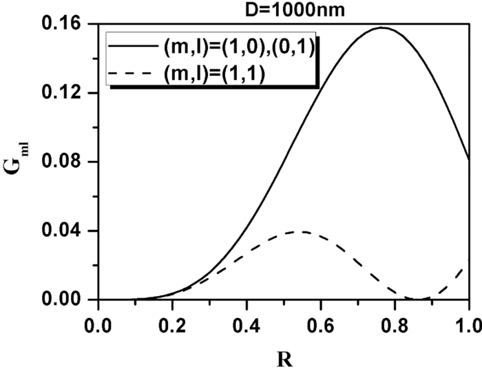
According to the model in Fig. 1, the Fourier transform of C(x,y,z) is Eq. 7[TeX:] \documentclass[12pt]{minimal}\begin{document}\begin{equation} C(x,y,z) = C_v \sum\limits_{m,l} {G_{ml} \exp (- i\mathord{\buildrel{\rightharpoonup} \over K} _{ml} } \cdot r) \end{equation}\end{document}
[TeX:]
\documentclass[12pt]{minimal}\begin{document}
\begin{equation*}
G_{ml} = \frac{{2d_1 }}{{D\sqrt {m^2 + l^2 } }}J_1 \left({\frac{{2\pi }}{D}d_1 \sqrt {m^2 + l^2 } } \right)
\end{equation*}
\end{document}
and J
1(x) is Bessel function. On the basis of the QPM theory,22 the periodical structure of collagen fibrils bundle causes an additional wave vector K
ml, which is
Eq. 8[TeX:] \documentclass[12pt]{minimal}\begin{document}\begin{equation} \mathord{\buildrel{\rightharpoonup} \over K} _{ml} = \frac{{2\pi m}}{D}\mathord{\buildrel{\rightharpoonup} \over z} + \frac{{2\pi l}}{D}\mathord{\buildrel{\rightharpoonup} \over y} \end{equation}\end{document}
[TeX:]
\documentclass[12pt]{minimal}\begin{document}
\begin{equation*}
\begin{array}{l}
\!\mathord{\buildrel{\rightharpoonup}
\over E} _2 (\theta,\varphi) {=} \displaystyle\sum\limits_{m,l} {\displaystyle\frac{{\nu C_v }}{r}(\sin ^2 \theta \sin ^2 \varphi {+} \cos ^2 \theta)^{1/2} }\int\!\!\!\!\int\!\!\!\!\int\frac{1}{2}\beta {G_{ml}E_{1}^{(0)2}} \\
\,\,\,\,\,\,\,\,\,\,\,\,\,\,\,\,\,\,\,\,\,\,\,\, \times \exp \left({ - 2\displaystyle\frac{{\mathord{\buildrel{\rightharpoonup}
\over x} ^{\lower3pt\hbox{$\scriptstyle 2$}} + \mathord{\buildrel{\rightharpoonup}
\over y} ^{\lower3pt\hbox{$\scriptstyle 2$}} }}{{w_{xy}^2 }} - 2\frac{{\mathord{\buildrel{\rightharpoonup}
\over z} ^{\lower3pt\hbox{$\scriptstyle 2$}} }}{{w_z }} + 2i\xi \frac{{n_1 }}{{n_2 }}k_1 \mathord{\buildrel{\rightharpoonup}
\over z} } \right) \\
\,\,\,\,\,\,\,\,\,\,\,\,\,\,\,\,\,\,\,\,\,\,\,\, \times \exp \bigg[ - ik_2 \bigg(z\cos \theta + y\sin \theta \sin \varphi + x\sin \theta \cos \varphi \\
\,\,\,\, \,\,\,\,\,\,\,\,\,\,\,\,\,\,\,\,\,\,\,\, +\, \displaystyle\frac{{2\pi m}}{{Dk_2 }}\mathord{\buildrel{\rightharpoonup}
\over z} + \frac{{2\pi l}}{{Dk_2 }}\mathord{\buildrel{\rightharpoonup}
\over y} \bigg) \bigg] \times dxdydz \\
\end{array}
\end{equation*}\end{document}
By integration,19
Eq. 9[TeX:] \documentclass[12pt]{minimal}\begin{document} \begin{equation} \mathord{\buildrel{\rightharpoonup} \over E} _2 (\theta,\varphi) = \sum\limits_{m,l} {C_w G_{ml} \mathord{\buildrel{\rightharpoonup} \over E} _2^{\lower3pt\hbox{$\scriptstyle \left(0 \right)$}} A\left({\theta,\varphi } \right)}, \end{equation}\end{document}
[TeX:]
\documentclass[12pt]{minimal}\begin{document}
\begin{equation*}
C_w = \left({\sqrt {\frac{\pi }{2}} } \right)^3 w_{xy}^2 w_z C_v,
\end{equation*}\end{document}
[TeX:]
\documentclass[12pt]{minimal}\begin{document}\begin{equation*}
\mathord{\buildrel{\rightharpoonup}
\over E} _2^{\lower3pt\hbox{$\scriptstyle (0)$}} = \frac{\nu }{r}(\sin ^2 \theta \sin ^2 \varphi + \cos ^2 \theta)^{1/2} \cdot \mathord{\buildrel{\rightharpoonup}
\over \mu } _2^{\lower3pt\hbox{$\scriptstyle (0)$}},
\end{equation*}\end{document}
[TeX:]
\documentclass[12pt]{minimal}\begin{document}\begin{equation*}
\mathord{\buildrel{\rightharpoonup}
\over \mu } _2^{\lower3pt\hbox{$\scriptstyle (0)$}} = \frac{1}{2}\mathord{\buildrel{\rightharpoonup}
\over E} _1^2 (0,0,0)\beta = \frac{1}{2}\mathord{\buildrel{\rightharpoonup}
\over E} _1^{\lower3pt\hbox{$\scriptstyle (0)2$}} \beta,
\end{equation*}\end{document}
which represent the contribution from the local induced polarization per unit volume density to the radiated electric field at the focal center only [indicated by the superscript (0)],
[TeX:]
\documentclass[12pt]{minimal}\begin{document}\begin{eqnarray*}
A (\theta,\varphi) &=& \exp \left\lbrace - \frac{{k_2^2 }}{8} \left[ w_{xy}^2 (\sin \theta \cos \varphi)^2\vphantom{w_z^2 \left(\cos \theta - \xi \displaystyle\frac{n_1 }{n_2 } + \frac{2\pi m}{Dk_2 } \right)^2}\right.\right.\nonumber\\
&& +\, w_{xy}^2 \left(\sin \theta \sin \varphi + \displaystyle\frac{2\pi l}{Dk_2 } \right)^2\nonumber\\
&&\left.\left. +\, w_z^2 \left(\cos \theta - \xi \displaystyle\frac{n_1 }{n_2 } + \frac{2\pi m}{Dk_2 } \right)^2 \right] \right\rbrace
\end{eqnarray*}\end{document}
According to the phase-match condition in SHG, when a particular order of (m,l) for K ml achieves perfect phase match, it would be the only order that contributes to the buildup of SHG while contributions from all others are neglected as the oscillating terms. Hence, the integral symbol in Eq. 9 can be ignored to be Eq. 10[TeX:] \documentclass[12pt]{minimal}\begin{document}\begin{equation} \mathord{\buildrel{\rightharpoonup} \over E} _2 (\theta,\varphi) = C_w G_{ml} \mathord{\buildrel{\rightharpoonup} \over E} _2^{\lower3pt\hbox{$\scriptstyle (0)$}} A\left({\theta,\varphi } \right). \end{equation}\end{document}2.5.Emission Direction of Second Harmonic Generation Electric FieldSHG detected along the parallel (||) and perpendicular (⊥) directions as the excitation polarization (α) are
[TeX:]
\documentclass[12pt]{minimal}\begin{document}\begin{equation*}
\begin{array}{l}
\!\!\left(\begin{array}{l}
\mathord{\buildrel{\rightharpoonup}
\over E} _2^{\lower3pt\hbox{$\scriptstyle ||$}} \\[3pt]
\mathord{\buildrel{\rightharpoonup}
\over E} _2^ {\lower3pt\hbox{$\scriptstyle \bot$}} \\[3pt]
\end{array} \right) \!\!=\! \left[ {
\begin{array}{*{20}c}
{\cos (\varphi - \alpha)} &\quad { - \sin (\varphi - \alpha)} \\[3pt]
{\sin (\varphi - \alpha)} &\quad {\cos (\varphi - \alpha)} \\[3pt]
\end{array}} \right]\left(
\begin{array}{l}
\mathord{\buildrel{\rightharpoonup}
\over E} _2^{\lower3pt\hbox{$\scriptstyle p$}} \\[3pt]
\mathord{\buildrel{\rightharpoonup}
\over E} _2^{\lower3pt\hbox{$\scriptstyle s$}} \\[3pt]
\end{array} \right) \\[3pt]
\,\,\,\,\,\,\,\,\,\,\,\,\,\,\,\,\, =\! C_w G_{ml} A\left({\theta,\varphi } \right) \!\left[\! {\begin{array}{*{20}c}
{\cos (\varphi {-} \alpha)} &\quad { {-} \sin (\varphi {-} \alpha)} \\[3pt]
{\sin (\varphi {-} \alpha)} &\quad {\cos (\varphi {-} \alpha)} \\[3pt]
\end{array}}\! \right]\left(\! \begin{array}{l}
\mathord{\buildrel{\rightharpoonup}
\over E} _2^{\lower3pt\hbox{$\scriptstyle (0)p$}} \\[3pt]
\mathord{\buildrel{\rightharpoonup}
\over E} _2^{\lower3pt\hbox{$\scriptstyle (0)s$}} \\[3pt]
\end{array}\! \right) \\[3pt]
\,\,\,\,\,\,\,\,\,\,\,\,\,\,\,\,\, =\! \displaystyle\frac{\nu }{r}C_w G_{ml} A\left({\theta,\varphi } \right)\!\left[\! {\begin{array}{*{20}c}
{\cos (\varphi {-} \alpha)} &\quad\!\!\!\!\! { {-}\! \sin (\varphi {-} \alpha)} \\[3pt]
{\sin (\varphi {-} \alpha)} &\quad\!\!\!\!\! {\cos (\varphi {-} \alpha)} \\[3pt]
\end{array}}\! \right]\! \cdot \mathord{\buildrel{\rightharpoonup}
\over M} \cdot\! \mathord{\buildrel{\rightharpoonup}
\over \mu } _2^{\lower3pt\hbox{$\scriptstyle (0)$}}, \\
\end{array}
\end{equation*}\end{document}
where
[TeX:]
$\mathord{\buildrel{\rightharpoonup}\over M}$
is the projection matrix, which permutes coordinate (x,y,z) to (θ,φ). Iτ ισ defined by
[TeX:]
\documentclass[12pt]{minimal}\begin{document}\begin{equation*}
\mathord{\buildrel{\rightharpoonup}
\over M} \left({\begin{array}{*{20}c}
{\mathord{\buildrel{\rightharpoonup}
\over \theta } } \\
{\mathord{\buildrel{\rightharpoonup}
\over \varphi } } \\
\end{array}} \right) = \left({\begin{array}{c@{\quad}c@{\quad}c}
{\cos \theta \cos \varphi } & {\cos \theta \sin \varphi } & { - \sin \theta } \\
{ - \sin \varphi } & {\cos \varphi } & 0 \\
\end{array}} \right).
\end{equation*}\end{document}
2.6.Second Harmonic Generation Emission PowerOn the basis of the formula of electric field presented in Eq. 9, the total power distribution of SHG thus has the following expression:19 Eq. 11[TeX:] \documentclass[12pt]{minimal}\begin{document} \begin{equation} P_2 (\theta,\varphi) = \frac{1}{8}n_2 \varepsilon _0 c\nu ^2 \beta ^2 \mathord{\buildrel{\rightharpoonup} \over E} _1^{\lower3pt\hbox{$\scriptstyle (0)4$}} C_w^2 G_{_{ml} }^2 H\left({\theta,\varphi } \right), \end{equation}\end{document}The power distribution in parallel (||) and perpendicular (⊥) components are
[TeX:]
\documentclass[12pt]{minimal}\begin{document}\begin{equation*}
\begin{array}{l} P_2^{||} (\theta,\varphi) = \displaystyle\frac{1}{2}n_2 \varepsilon _0 cr^2 |\mathord{\buildrel{\rightharpoonup}\over E} _2{\lower3pt\hbox{$\scriptstyle ||$}} (\theta,\varphi)|^2 \\[8pt]
\,\,\,\,\,\,\,\,\,\,\,\,\,\,\,\,\,\,\,\,\,\,\, = \displaystyle\frac{1}{8}n_2 \varepsilon _0 cG_{ml}^2 \nu ^2 C_w^2 A^2 (\theta,\varphi)\mathord{\buildrel{\rightharpoonup}\over E} _1^{\lower3pt\hbox{$\scriptstyle (0)4$}}, \\ \end{array}
\end{equation*}\end{document}
Eq. 12[TeX:] \documentclass[12pt]{minimal}\begin{document} \begin{eqnarray} &&\{ \cos (\varphi - \alpha)[\cos \theta \cos \varphi (\beta _{xxx} \cos ^2 \alpha + \beta _{xyy} \sin ^2 \alpha) \nonumber\\ &&\quad +\, \beta _{xyy} \cos \theta \sin \varphi \sin 2\alpha]-\, \sin (\varphi - \alpha) \nonumber\\ &&\quad\times [ - \sin \varphi (\beta _{xxx} \cos ^2 \alpha + \beta _{xyy} \sin ^2 \alpha) \nonumber\\ && \quad +\, \beta _{xyy} \cos \varphi \sin 2\alpha]\} ^2, \end{eqnarray}\end{document}
[TeX:]
\documentclass[12pt]{minimal}\begin{document}
\begin{equation*}
\begin{array}{l}
P_2^ \bot (\theta,\varphi) = \displaystyle\frac{1}{2}n_2 \varepsilon _0 cr^2 |\mathord{\buildrel{\rightharpoonup}
\over E} _2^ {\lower3pt\hbox{$\scriptstyle \bot$}} (\theta,\varphi)|^2 \\[6pt]
\,\,\,\,\,\,\,\,\,\,\,\,\,\,\,\,\,\,\,\,\,\,\, = \displaystyle\frac{1}{8}n_2 \varepsilon _0 cG_{ml}^2 \nu ^2 C_w^2 A^2 (\theta,\varphi)\mathord{\buildrel{\rightharpoonup}
\over E} _1^{\lower3pt\hbox{$\scriptstyle (0)4$}}, \\
\end{array}
\end{equation*}
\end{document}
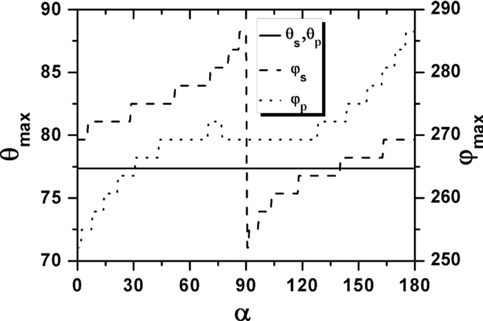
Eq. 13[TeX:] \documentclass[12pt]{minimal}\begin{document} \begin{eqnarray} && \{ \sin (\varphi - \alpha)[\cos \theta \cos \varphi (\beta _{xxx} \cos ^2 \alpha + \beta _{xyy} \sin ^2 \alpha) \nonumber\\ &&\quad +\, \beta _{xyy} \cos \theta \sin \varphi \sin 2\alpha] +\, \cos (\varphi - \alpha) \nonumber\\ &&\quad\times [ - \sin \varphi (\beta _{xxx} \cos ^2 \alpha + \beta _{xyy} \sin ^2 \alpha) \nonumber\\ &&\quad +\, \beta _{xyy} \cos \varphi \sin 2\alpha]\} ^2. \end{eqnarray}\end{document}3.Theoretical Simulation Study of Effects of Parameters on Second Harmonic Generation Emission AngleIn Eq. 11, P 2(θ,φ) ∝ β2 indicates that the biophysical feature (denoted by β) of constituted collagen dipoles will only affect the total amount of SHG emission power rather than the power distribution along SHG emission angle (θ,φ). In this paper, because we focus on the exploration of the parameters that may influence the SHG emission angle (θ,φ), the effect of β is ignored and we make the following assumptions to simplify our model in this section. First, the ratio of the fibrils diameter to the collagen period is defined to be R = d 1/D = 1/2, which indicates the water interval d 2 has the same size with fibrils diameter d 1 = (d 2 = d 1) as shown in Fig. 1b. Second, a fixed value λ1 = 800 nm is applied in our following simulations because, usually, the excitation wavelengths λ1 that most experiments take for SHG in biological applications are between 700 and 1000 nm. Third, the coefficient [TeX:] $(1/8)n_2 \varepsilon _0 c\nu ^2 E_1^{(0)4}$ is normalized to be 1. 3.1.Effects of Numerical Aperture on Second Harmonic Generation Emission AngleFigure 2a demonstrates the peak SHG emission angle (θmax,φmax) when the SHG emission power is maximum P 2max, which implies the optimizing SHG imaging angle as NA changes from 0.2 to1.2 under the condition of collagen period of D = 500 nm (d 1 = 250 nm), (m,l) = (1,0), and α = 0 deg. We note that as NA increases from 0.2 to 1.2, θmax increases from 65 to 76 deg, while θmax always keeps in direction of +90 or –90 deg, indicating the emission direction of the maximum P 2max is confined in the yz plane when α = 0 deg. NA has also been found to have influence on the total SHG emission power P 2, as demonstrated in Fig. 2b. It has a greater impact on P 2 within the range of 0.8–1.2 than that of 0.2–0.8, in which its influence is negligible. Hence, NA = 0.8 is chosen for our following discussions, where it is necessary. Figure 2c shows the variation of θmax with the collagen period D at NA 0.4, 0.8, and 1.2 under the order (m,l) = (1,0) and α = 0 deg. It shows that all SHG emission has symmetrical characteristics that locate opposite the direction of the excitation light (θ = 180 deg). Furthermore, we note that the influence of NA on θmax at different collagen period D does not make much difference. Compared to NA, collagen period D obviously has more of an impact on SHG emission angle θmax; thus, it is explored in more detail in Sec. 3.3. 3.2.Effects of Structural Order (m,l) on Second Harmonic Generation Emission AngleThe 3-D distribution of SHG emission angles (θ,φ) under two collagen periods D = 150 nm (d 1 = 75 nm) and D = 1000 nm (d 1 = 500 nm) when α = 0 deg with structural orders (m,l) = (1,0), (0,1), and (1,1), respectively, are demonstrated in Fig. 3. It shows that the peak emission angle φmax keeps the same value through all the orders and collagen periods, which is 90 deg and/or 270 deg (in the [TeX:] $\hat y - \hat z$ plane) under the excitation conditions. On the other hand, the peak emission angle θmax presents different patterns on D and (m,l). We note that there are two emission lobes of SHG when (m,l) = (1,0), whereas at other demonstrated cases, only one emission lobe exists. Furthermore, we find that when D = 1000 nm, although under the case of (m,l) = (1,0), there are two SHG emission lobes, the emission power of these two lobes are much lower than that of D = 150 nm, which means, in practice, it could be undetectable. Also, under the structural order of (m,l) = (0,1) and (m,l) = (1,1), if the fibrils diameter D is smaller, such as D = 150 nm, then the only one emission lobe has much lower power to be detected. Fig. 3SHG emission power distribution of (θ,φ) varies with two fibrils periods D = 150 nm and D = 1000 nm under the most commonly involved three structural orders (m,l) = (1,0), (m,l) = (0,1), and (m,l) = (1,1). 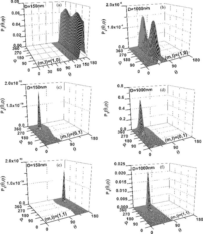 The key point that attracts our attention in Fig. 3 is that when D is relatively smaller, such as D = 150 nm, under both (m,l) = (1,0) and (1,1), SHG emission presents the backward emission (θmax > 90 deg). However, at (m,l) = (0,1), SHG emission presents the forward feature (θmax < 90 deg). This result indicates that the structure character of collagen fiber along the incident light direction [TeX:] $\mathord{\buildrel{\rightharpoonup}\over z}$ , which is characterized by the parameter m, plays the major role on backward emission of SHG. When D is relatively bigger, for example, D = 1000 nm, SHG presents forward emission under all three (m,l) orders. 3.3.Effects of Collagen Period D on Second Harmonic Generation Emission AngleRealizing that the collagen period D plays an important role on the peak SHG emission angle θmax, the impact of collagen period D from 100 to 1000 nm on the peak SHG emission angle under different orders (1,0), (0,1), and (1,1) in the case of NA = 0.8 and thus has correspondingly been demonstrated in Fig. 4a. With the structural order (1,0) and (1,1), θmax drops dramatically from starting angle 180 deg at first and then decreases slowly after it crosses 90 deg (nonlinear). There is a threshold value of collagen period D, in our case it is ∼300 nm. When D is smaller than this value, the backward emission of SHG occurs (θmax > 90 deg); otherwise, SHG emits along the forward direction (θmax < 90 deg). When the structural order (m,l) is (0,1), on the contrary, only two peak SHG emission angles denoting forward emission of either 26 deg (D < 200 nm) or 37 deg (D ≥ 200 nm) along all sizes of D are induced. The variation of θmax as D is not smoothly, there is a quantum leap as shown in the inserted figure. To further understand the functions of D on SHG emission, the effect of D on the total SHG emission power (P 2) under different cases of structural orders (m,l) are correspondingly shown in Fig. 4b. Note that as the collagen period D is >350 nm (relative larger size of D), the emission power of SHG under structural order (0,1) takes superior contribution over others to total SHG emission power. When 170 < D < 350 nm (middle size of D), the emission power of SHG under structural order (1,1) plays dominant role. Although structural order (1,0) has its dominant contribution when the range of D falls between 100 and 170 nm. Figure 4b clearly demonstrates that the structural feature of collagen fiber [determined by structural order (m,l)] will play a role only on a certain range of collagen period D or fibrils diameter d 1. 3.4.Effects of Polarization Angle α of Fundamental Light n Second Harmonic Generation Emission AngleThe effects of polarization angle α on peak SHG emission angles is taken into account, as shown in Fig. 5 [Eqs. 12, 13]. Here, the collagen period is assumed to be D = 400 nm and the first hyperpolarizabilities to be βxyy = 1 and βxxx = 2.6. Because the polarization angle α varies from 0 to π, we note that the peak angles (θs,θp) corresponding to the maximum perpendicular and parallel emission power keep stable values (θs = θp is ∼77 deg). While the peak angle φmax, on the other hand, has an obvious change. The peak angle φs corresponding to the maximum perpendicular SHG power increases with α and appears a distinct transit around α = 90 deg. The peak angle φp corresponding to the maximum parallel SHG emission power almost keeps constant when α is between 50 and 130 deg. The changes of the emission angle as the polarization angle α have the same feature of quantum leap as that of φmax along D, as shown in Fig. 4a. 4.Conclusions and DiscussionsAccording to the structural characteristics of collagen type I fiber, which is constituted by fibrils in a square quasi-crystalline formation, the density distribution function C(x,y,z) describing the distribution of dipoles in such crystallized fibrils bundle and structural order (m,l) characterized by QPM theory is introduced in this paper to deal with the SHG emission from collagen fiber. The effects of NA, structural order (m,l), collagen period D = d 1 + d 2, as well as polarization angle α on emission angles of SHG have been investigated. NA has influence on SHG emission angle, such as the increase of NA causes an increase of the peak emission angle θmax and the total SHG emission power, but for different D, the difference is slight. We have made a detailed investigation of collagen period D on SHG emission in this paper. Because D = d 1 + d 2, to utilize the results to get an intuitive understanding of the fibrils diameter d 1 on SHG emission, we assume that d 1 = D/2 here. This assumption is reasonable if we are only interested in the effects of d 1 on the SHG emission angle. The ratio of fibrils diameter to collagen period (R = d 1/D), without a doubt, has an influence on G ml, as shown in Fig. 6. However, based on Eq. 9, we know that G ml would only affect the total amount power of SHG rather than the emission angle and the corresponding power distribution. Therefore, d 1 = D/2 (R = 1/2) is made when we analyze the effect of d 1 on θmax based on the results of D. Our investigations show that, when the diameter of fibrils d 1 decreases, for the same structural order, for example, (m,l) = (1,0) or (1,1) and at the same NA, the θmax increases correspondingly. As the diameter of fibrils d 1 reaches a threshold value, which in our case is around d 1 = 150 nm, backward SHG emission appears [Fig. 4a]. The relationship of forward/backward emission of SHG with the fibril's diameter has been supported by previous experimental results. It has been shown that there are more striking SHG backward images than the forward from fibril segments of immature two-day-old rat-tail tendon,16 which is predominated by immature fibrils (small diameter of fibrils8). Also, in 10-day-old rat-tail tendon, they verify that the immature fibril segments scatter backward, whereas mature fibril segments (the large diameter of fibrils8) is forward.24 Our simulation results of SHG backward emission has been further verified by the experimental results of forward to backward (F/B) ratio of SHG to fibril diameter.16 There, the diameter of fibrils is modulated by the NaCl concentration; the higher of the NaCl concentration is, the smaller the fibrils size is due to shrinkage. The experimental results clearly show that the F/B ratio obviously decrease with the decrease of fibril size induced by an increase of NaCl concentrations. Our simulation results regarding the effects of structural order (m,l) indicate that the structural feature of collagen fiber along the incident light direction [TeX:] $\mathord{\buildrel{\rightharpoonup}\over z}$ , which is characterized by the parameter m, plays a major role on backward emission of SHG because the fibril diameter is small enough (Fig. 3), where (m,l) = (1,0) and (1,1) makes the backward SHG emission happen when D = 150 nm; however, (m,l) = (0,1) makes SHG emission keep the forward direction. Furthermore, Fig. 4 shows that θmax has little difference between structural order (1,0) and (1,1) as the variation of D, which also indicates that, compared to m,l, has a minor effect on the determination of θmax. In other words, the structure feature along the incident light direction has the dominant effect on θmax to be forward or backward. Fig. 4(a) Effect of fibrils period D at different (m,l) on peak SHG emission angle θmax. (b) SHG total emission power as varied fibrils period D at different (m,l).  Additionally, the simulation results demonstrated in Figs. 3 and 4b indicate that, under the certain structural features represented by (m,l), such as (m,l) = (1,0), there are two symmetrical emission lobes along all the collagen periods D (Fig. 3). However, if this structural feature does not function on those collagen periods D, here, for example, D = 1000 nm, which is out of the scope (100–170 nm), where the structural order (m,l) = (1,0) has its dominant contribution [Fig. 4b], the emission power produced from the collagen fiber with those collagen periods would be very low; the two emission lobes appear theoretically would not exist in practice [Figs. 3b and 3c]. In other circumstances, such that the collagen fiber satisfies the structural feature of (m,l) = (0,1) or (m,l) = (1,1), it is possible to have only one emission lobe of SHG [Figs. 3c, 3d, 3e, 3f]. However, Fig. 4b indicates that if the collagen fiber period D falls in the range of the overlapping functional area of (m,l) = (0,1) and (1,1), both structural features may have their contributions to the SHG emission; therefore, two SHG emission lobes would still be expected, but the emission power of those two lobes could be unbalanced. From our simulation results in Fig. 5, we realize that fundamental wave polarization angle α has no influence on θmax but on φmax. Our theoretical simulation results of the optimizing SHG imaging angle (θmax,φmax) with the relationship of the NA, collagen structure order (m,l), fibrils diameter d 1, and the polarization angle α of the incident laser would be very helpful on the optimization of experimental protocols for efficient SHG imaging. AcknowledgmentsThe authors gratefully thank the National Natural Science Foundation of China (Grants No. 30470495 and No. 30940020) for their support. ReferencesP. J. Campagnola and
L. M. Loew,
“Second-harmonic imaging microscopy for visualizing biomolecular arrays in cells, tissues and organisms,”
Nat. Biotechnol., 21 1356
–1360
(2003). https://doi.org/10.1038/nbt894 Google Scholar
F. Helmchen and
W. Denk,
“Deep tissue two-photon microscopy,”
Nat. Methods, 2
(12), 932
–940
(2005). https://doi.org/10.1038/nmeth818 Google Scholar
L. Moreaux, O. Sandre, and
J. Mertz,
“Membrane imaging by second-harmonic generation microscopy,”
J. Opt. Soc. Am. B, 17 1685
–1694
(2000). https://doi.org/10.1364/JOSAB.17.001685 Google Scholar
I. Freund and
M. Deutsch,
“Second-harmonic microscopy of biological tissue,”
Opt. Lett., 11 94
–96
(1986). https://doi.org/10.1364/OL.11.000094 Google Scholar
G. Cox, E. Kable, A. Jones, I. Fraser, F. Manconi, and
M. D. Gorrell,
“3-Dimensional imaging of collagen using second harmonic generation,”
J. Struct. Biol., 141 53
–62
(2003). https://doi.org/10.1016/S1047-8477(02)00576-2 Google Scholar
D. J. Prockop and
A. Fertala,
“The collagen fibril: the almost crystalline structure,”
J. Struct. Biol., 122 111
–118
(1998). https://doi.org/10.1006/jsbi.1998.3976 Google Scholar
P. Fratzl and
R. Weinkamer,
“Nature's hierarchical materials,”
Prog. Mater. Sci., 52 1263
–1334
(2007). https://doi.org/10.1016/j.pmatsci.2007.06.001 Google Scholar
D. A. D. Parry, G. R. G. Barnes and
A. S. Craig,
“A comparison of the size distribution of collagen fibrils in connective tissues as a function of age and a possible relation between fibril size distribution and mechanical properties,”
Proc. R. Soc. London, Series B, 203 305
–321
(1978). https://doi.org/10.1098/rspb.1978.0107 Google Scholar
S. J. Lin, S. H. Jee and
C. Y. Dong,
“Multiphoton microscopy: a new paradigm in dermatological imaging,”
Eur. J. Dermatol., 17 361
–366
(2007). https://doi.org/10.1684/ejd.2007.0232 Google Scholar
A. M. Raja, S. Xu, W Sun, J. Zhou, D. C. Tai, C. S. Chen, J. C. Rajapakse, P. T. So, and
H. Yu,
“Pulse-modulated second harmonic imaging microscope quantitatively demonstrates marked increase of collagen in tumor after chemotherapy,”
J. Biomed. Opt., 15
(5), 056016
(2010). https://doi.org/10.1117/1.3497565 Google Scholar
V. A. Hovhannisyan, P. Su, S. Lin, and
C. Dong,
“Quantifying thermodynamics of collagen thermal denaturation by second harmonic generation imaging,”
Appl. Phys. Lett., 94 233902
(2009). https://doi.org/10.1063/1.3142864 Google Scholar
S. Psilodimitrakopoulos, V. Petegnief, G. Soria, I. Amat-Roldan, D. Artigas, A. M. Planas, and
P. Loza-Alvarez,
“Polarization second harmonic generation (PSHG) imaging of neurons: estimating the effective orientation of the SHG source in axons,”
Proc. SPIE, 7569 75692W
(2010). https://doi.org/10.1117/12.841313 Google Scholar
S. Psilodimitrakopoulos, V. Petegnief, G. Soria, I. Amat-Roldan, D. Artigas, A. M. Planas, and
P. Loza-Alvarez,
“Estimation of the effective orientation of the SHG source in primary cortical neurons,”
Opt. Express, 17 14418
–14425
(2009). https://doi.org/10.1364/OE.17.014418 Google Scholar
F. Tiaho, G. Recher, and
D. Rouède,
“Estimation of helical angles of myosin and collagen by second harmonic generation imaging microscopy,”
Opt. Express, 15 12286
–12295
(2007). https://doi.org/10.1364/OE.15.012286 Google Scholar
X. Y. Deng, E. D. Williams, E. W. Thompson, X. Gan, and
M. Gu,
“Second-harmonic generation from biological tissues: effect of excitation wavelength,”
Scanning, 24 175
–178
(2002). https://doi.org/10.1002/sca.4950240403 Google Scholar
R. M. Williams, W. R. Zipfel, and
W. W. Webb,
“Interpreting second-harmonic generation images of collagen I fibrils,”
Biophys. J., 88 1377
–1386
(2005). https://doi.org/10.1529/biophysj.104.047308 Google Scholar
F. Legare, C. Pfeffer, and
B. R. Olsen,
“The role of backscattering in SHG tissue imaging,”
Biophys. J., 93 1312
–1320
(2007). https://doi.org/10.1529/biophysj.106.100586 Google Scholar
S. M. Zhuo, J. X. Chen, G. Z. Wu, S. S. Xie, L. Q. Zheng, X. S. Jiang, and
X. Q. Zhu,
“Quantitatively linking collagen alteration and epithelial tumor progression by second harmonic generation microscopy,”
Appl. Phys. Lett., 96 213704
(2010). https://doi.org/10.1063/1.3441337 Google Scholar
Y. Chang, C. S. Chen, J. X. Chen, Y. Jin, and
X. Y. Deng,
“Theoretical simulation study of linearly polarized light on microscopic second-harmonic generation in collagen type I,”
J. Biomed. Opt., 14 044016
(2009). https://doi.org/10.1117/1.3174427 Google Scholar
R. LaComb, O. Nadiarnykh, S. S. Townsend, and
P. J. Campagnola,
“Phase matching considerations in second harmonic generation from tissues: effects on emission directionality, conversion efficiency and observed morphology,”
Opt. Commun., 281 1823
–1832
(2008). https://doi.org/10.1016/j.optcom.2007.10.040 Google Scholar
G. A. Magel, M. M. Fejer, and
R. L. Byer,
“Quasi-phase-matched second harmonic generation of blue light in periodically poled LiNbO3,”
Appl. Phys. Lett., 56 108
–110
(1990). https://doi.org/10.1063/1.103276 Google Scholar
M. M. Fejer, G. A. Magel, D. H. Jundt, and
R. L. Byer,
“Quasi-phase-matched second harmonic generation: tuning and tolerances,”
IEEE J. Quantum Electron., 28 2631
–2654
(1992). https://doi.org/10.1109/3.161322 Google Scholar
L. Tian, J. L. Qu, Z. Y. Guo, Y. Jin, Y. Y. Meng, and
X. Y. Deng,
“Microscopic second-harmonic generation emission direction in fibrillous collagen type I by quasi-phase-matching theory,”
J. Appl. Phys., 108 054701
(2010). https://doi.org/10.1063/1.3474667 Google Scholar
W. R. Zipfel, R. M. Williams, and
W. W. Webb,
“Nonlinear magic: multiphoton microscopy in the biosciences,”
Nat. Biotechnol., 21 1368
–1376
(2003). https://doi.org/10.1038/nbt899 Google Scholar
E. Hecht, Optics, Higher Education Press, Beijing
(2005). Google Scholar
|