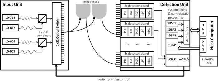2.1.

Light Input Unit

The input unit is responsible for generating the light with which the target will be illuminated. The system uses four wavelengths of near-infrared light at 765, 808, 827, and 905 nm generated by continuous-wave high power laser diodes (HPD-1010-HHLF-TEC, High Power Devices, Inc.). Each laser diode is controlled by a laser driver controller (ITC110, Thorlabs Inc.) and modulated with an input current at either 5 kHz (765 and 808 mm) or 7 kHz (827 and 905 nm). Modulating the laser light intensity allows for simultaneous illumination of the target with multiple wavelengths as well as the rejection of ambient light. The four wavelengths are passed through two wave-division multiplexers (Oz Optics Ltd.) to create two separate streams of light: one stream that combines 765 nm modulated at 5 kHz and 827 nm modulated at 7 kHz, and one stream that combines 808 nm modulated at 5 kHz and 905 nm modulated at 7 kHz. Due to the fact that each stream must be detected with the same hardware, the same amount of gain must be applied to all wavelengths of the stream. In cases where the attenuation through the tissue is significantly different at the various wavelengths, it can be difficult to find one gain setting to accommodate all four wavelengths. Thus, our design uses two streams of light with two wavelengths in each stream that tend to experience similar attenuation. Each modulation frequency is generated by a direct digital synthesis (DDS) chip (AD9854, Analog Devices Inc.) and passed through a series of filters as well as offset and amplitude adjustment stages prior to being input to the laser driver controller. The output frequency of the DDS chip is controlled by a programmable microcontroller (AT89S8253, Atmel).

The two light streams are passed into a 2 × 32 optomechanical switch (Sercalo Rack System Solutions, RS-FSPA 2×1×32-62FCPC). The switch begins by illuminating the target at one source position with the first wavelength set (765 and 827 nm) and then the second wavelength set (808 and 905 nm) before moving onto the next source position. It continues this source switching until all programmed source positions (up to 32 per breast) have illuminated the target. The switching is customizable so that the system can run with only two wavelengths twice as quickly since it does not need to repeat the measurements at each source position a second time for the additional wavelength set. The optical switch takes less than 7 ms to settle when switching between positions.

Multimode 62/125 optical fibers leave the switch and then bifurcate to simultaneously illuminate both the left and right breast with 4-mm-diameter tips. The fibers are brought into contact with the breast using a hand-like measuring apparatus developed by NIRx Medical Technologies, shown in Fig. 2. In the measuring apparatus, 16 sources and 16 detectors are arranged in a flat geometry beneath the breast, while the other 16 sources and 16 detectors are brought into contact with the top of the breast with eight adjustable fingers, each one holding four fibers. All sources are co-localized with detector fibers, giving each breast a total of 64 detectors and 32 sources. The setup is designed to minimize patient discomfort by imaging without compression and with the patient in a comfortable seated or standing position.

Fig. 2

Photograph of the interface used to bring the optical fibers in contact with the breast. Articulating fingers bring 32 fibers into contact with the top portion of the breast, while 32 fibers arranged in a flat geometry make contact with the bottom portion of the breast. Half of the fibers are both sources and detectors while the other half are dedicated detectors.

2.2.

Light Detection Unit

The light detection unit is the key component of the system as its design allows for the fast collection and processing of large amounts of data. An overview of the interactions between the various boards and chips that make up the detection unit is presented in Fig. 3. The detection unit starts with analog circuitry to amplify and filter the signal prior to quantization with an analog-to-digital converter (ADC). The ADC interacts with a complex programmable logic device (CPLD) and DSP chip that work to acquire the signal, demodulate the signal to extract the amplitude, and pass the amplitude onto the host computer via data acquisition cards. The DSP and CPLD chips also coordinate the timing of the system and keep the various components synchronized while optimizing the system performance. Power to the detection unit is provided by a compact peripheral component interconnect (PCI) power supply (Chroma cPWR-59401) that provides voltage rails at +5, +3.3, +12, and −12 V.

Fig. 3

Overview of the detection circuitry and logic showing the interaction between the DSP master board, DSP slave board, detection boards, and host computer.

2.2.1.

Analog detection electronics

The analog portion of the detection unit involves converting the detected photons into an electronic signal and then conditioning that signal in preparation for digitization. The first stage of the analog electronics consists of a silicon photodiode (Si-PD: Hamamatsu S1337–33BR) that converts the incident photons into a current that is then amplified and output as a voltage using a trans-impedance amplifier (TIA). The trans-impedance amplifier uses a bandwidth extension technique to enable high gain and sufficient bandwidth for the 5 and 7 kHz signals that must be amplified.³⁵ Following the TIA, a passive RC high-pass filter removes the DC component of the signal. From there, the signal passes through a second gain stage referred to as the programmable gain amplifier (PGA) that provides additional amplification, but no additional signal-to-noise ratio (SNR). The PGA is primarily responsible for bringing the signal into a suitable range for detection with the ADC.

To control the resistor values across the TIA and the PGA gain stages, three bits are used to encode a range of gain settings. The resistor values for the TIA range from 10 kΩ to 100 MΩ and the PGA gain ranges from 1 to 100. The three gain bits control the resistor value for the TIA and PGA via a multiplexer and reed relays that are used to switch between the values. The available gain bits and their TIA and PGA gain are shown in Table 1. The gain bits can be manually controlled through the host computer user interface or through an automatic detection routine that will test and select the optimal settings. The optimal setting is determined as the best SNR without saturation. The host computer passes the gain bits to the DSP through a series of shift registers that daisy-chain through the detection boards. Once all of the gain bits have been chained through the boards, a signal transfers the gain bits into a first-in-first-out (FIFO) buffer for storage on each detection board. During imaging, as the source position is changed, the new gain bit settings are read out locally from the FIFO thereby quickly modifying the resistor values across the TIA and PGA.

Fig. 12

DOT images for case study 3, a healthy patient. (a) 3D isosurface taken at 3% d[Hb] identifies no tumor region in either breast. (b) Location of 2D slices extracted from the 3D reconstruction. Finally, the 2D maps of d[HbO₂]% (top row) and d[Hb]% (bottom row) are shown for the (c) left and (d) right breasts.

Table 1

Description of the detection gain settings.

Gain setting	Overall gain (V/A)	TIA gain (V/A)	PGA gain (V/V)
1	10 k	10 k	1
2	100 k	10 k	10
3	1 M	10 k	100
4	10 M	10 M	1
5	100 M	10 M	10
6	1 G	10 M	100
7	10 G	100 M	100

Following the TIA and PGA gain stages, the signal is filtered with an eighth-order Butterworth anti-aliasing filter that removes high-frequency components and whose primary purpose is to ensure that there are no frequencies present above the Nyquist frequency prior to digitization. The signal is sampled at 75 ksamples/s, which means that the Nyquist frequency is 37.5 kHz. As a result, we choose a cutoff frequency of 12.5 kHz and a Butterworth filter that has a flat passband for the 5 and 7 kHz signals, while also providing strong attenuation of any higher frequency noise at risk of aliasing into the passband. Furthermore, an operational amplifier offsets the signal so that it is centered around 2.5 V in order to take advantage of the full 0 to 5 V input range of the ADC.

Finally, the signal is brought into the digital domain using a four channel, 16-bit, successive approximation register ADC (AD7655, Analog Devices Inc.) that samples at a maximum rate of 1 Msamples/s. In our system, the ADC samples the data from each detector channel at 75 kHz. The ADC timing is synchronized with the rest of the digital electronics through the master CPLD and DSP.

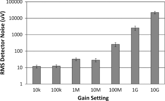
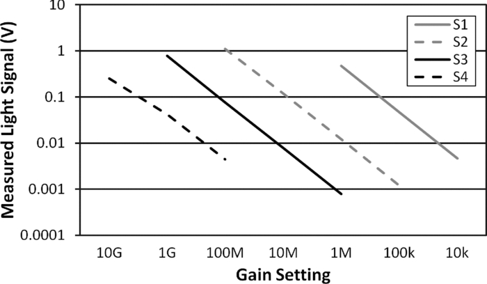
2.2.4.

System timing

To obtain fast imaging speeds, it is important to have careful coordination between the various components of the system, while also accounting for the settling times of the electronics and optical switch. There are many occasions where the system multi-tasks to optimize the imaging speed. The system timing is outlined in detail in Fig. 4.

Fig. 4

Detailed timing sequence outlining the synchronization between the optical switch, ADC, and DSP to acquire one frame of data.

The DSPs acquire 150 samples from each of the 128 detectors over a period of 2 ms so that each detector is effectively sampled at 75 ksamples/s. The chip select (CS) signal sequentially selects two ADCs per DSP at a time to pass the digitized samples onto that DSP. Each 16-bit ADC can digitize two channels at a time and passes them onto the DSP as one 32-bit packet. For example, mDSP first receives sample 1 from channels 1&3 of ADCs 1&2, followed by sample 1 from channels 1&3 of ADCs 3&4, followed by sample 1 from channels 1&3 of ADCs 5&6, and finally sample 1 from channels 1&3 of ADCs 7&8. It then proceeds to acquire sample 1 from channels 2&4 from each set of ADCs before moving onto the next sample. In parallel, sDSP1, sDSP2, and sDSP3 are receiving data from ADCs 9 through 32. The sCPLD is responsible for coordinating the routing of the ADC data to the appropriate DSP in each cycle, as coordinated by the CS signal.

Once the DSPs have received 150 samples from all 128 detectors, the mDSP signals to the mCPLD to change the source position and begins the 7 ms pause waiting for the switch to settle. During that settling time, the speed of the system is optimized by having the DSPs run the lock-in detection on the samples from the previous source before sending them out to the host computer. In addition, while the optical switch is settling on the new source position, the gain bits are updated, and the analog electronics have time to settle.

2.3.

Host Computer and User Interface

The host computer uses a LabVIEW graphical user interface (GUI) to facilitate communication with the hardware. The system can be configured through the GUI to run with an arbitrary number of sources and detectors and wavelengths. The GUI gives the user the ability to manually configure the gain settings for each source-detector pair, but also provides the ability to automatically test and select optimal gain settings for each source and detector. Once the optimal gain settings are selected, the imaging screen provides the ability to start, pause, and stop imaging. It also shows the real-time traces of the detector signals for a given source and wavelength. Screen shots of the user interface to control the gain bit settings and the image acquisition are shown in Fig. 5.

Fig. 5

Screenshots of the LabVIEW user interface to (a) control the gain bits for each source-detector pair and (b) visualize the raw data as it is acquired.

3.1.

System Timing

This system was designed for dynamic breast imaging, making the dynamic range and the speed of acquisition two of the primary criteria. The temporal response, as described in detail in Sec. 2.2.4, is limited by the settling time of the optical switch and the number of source positions and wavelengths. The switch requires 7 ms to settle after switching positions, followed by 2 ms to acquire the data for all detectors at that source position. This brings the imaging time to 9 ms per source position. Since we sequentially image the two wavelength sets, the imaging rate also depends on the number of wavelengths. Consequently, the fastest that the system can image is to collect one frame in 0.009 s with one source and two wavelengths (111 Hz). Or, with 32 sources and two wavelengths it can acquire a frame in 0.288 s (3.5 Hz). Finally, the slowest configuration is to use all 32 sources and four wavelengths, in which case it takes 0.576 s to acquire one frame (1.7 Hz).

3.2.

Dark Noise

The dark noise is the measured signal when no incident light is present, and thus represents the smallest measurement that can be reliably made with the system. Figure 6 shows the dark noise measured for each gain setting with the standard deviation of the measurements across all detectors indicated by the error bars. As expected, with increasing amplification in the PGA stage, and eventually in the TIA stage, we see increasing noise present. At the lower gain stages we see noise levels below 50 μV, but as the gain increases we see increasing noise; until at the highest gain stage of 10 GV/A, we have an RMS dark noise of 22 mV. The slightly higher noise at the 1 M versus the 10 M setting represents the fact that the 1 M setting uses less TIA gain and more PGA gain, whereas the 10 M setting uses more TIA gain and less PGA gain. While TIA gain improves the SNR, PGA gain does not. This finding demonstrates that increasing the gain at the TIA stages is preferred over increasing the gain at the PGA stage.

Fig. 6

Logarithmic plot of the RMS dark noise for each detector gain setting.

3.3.

Noise Equivalent Power and Dynamic Range

The noise equivalent power (NEP) is an indication of the detector sensitivity to light and can be computed for an SNR of unity using the dark noise of the highest gain setting. Taking the mean of the root-mean-squared (RMS) detector noise at the highest gain setting and using the known properties of the silicon photodetector in the given wavelength range of 0.5 W/A, we calculate that the NEP is approximately 4.5 pW RMS. The NEP represents the smallest light signal that can be detected. The largest light signal that can be detected uses the full detector range for the lowest gain setting, which in this case is to detect 2.5 V peak-to-peak on the 10 kV/A gain setting. Using these values we can calculate the dynamic range of the system to be 10⁸ (or 158 dB).

3.4.

Coefficient of Variation and Long Term Stability

The coefficient of variation (CV) is calculated here for a static breast-shaped phantom with breast optical properties over a period of five minutes (500 frames) with the full number of sources and detectors. Figure 7 shows the mean of the CV calculated for all detectors at the given gain setting for each wavelength. Up until 100 MV/A, the CV is as low as 0.15% for some wavelengths but by the highest gain setting it increases to approximately 3%. The SNR for each of these settings can be calculated as 20log₁₀(1/CV) giving us an average SNR of 51 dB for the lowest gain setting and 30 dB for the highest gain setting.

Fig. 7

Mean CV of the detectors at each gain setting for each wavelength with standard deviation error bars.

To assess the long term stability of the system, we measured the same static breast phantom over 40000 frames (∼38 min). Taking the mean of measured values at frame 1 and calculating the percentage change between that and the mean at frame 40000, there is a 0.7% change in the measured value.

3.5.

System Linearity

System linearity was examined by using the same incident light on a detector and then measuring the detected voltage across all possible gain settings. This was repeated four times in order to cover all gain settings and the results are plotted in Fig. 8, where we see that a linear relationship across the gain settings is generally maintained. We expect to see a 10× gain factor between each gain setting measuring the same signal. An exponential fit of the data in Fig. 8 should give an equation of e^−2.3 in a perfectly linear 10× relationship between gain settings. For the curves below, we see good linearity with fits of e^−2.31 (R = 1), e^−2.27 (R = 0.9999), e^−2.30 (R = 1), and e^−2.02 (R = 0.9955) for S1 through S4. We expect the decreased linearity at the highest gain settings (reflected by S4), since those settings also introduce higher noise levels.

Fig. 8

Linearity across all gain settings measured through four samples (S1 to S4) covering all settings. Each sample reflects the same input intensity measured across multiple gain settings.

3.6.

System Summary and Discussion

The various system characteristics are summarized in Table 3. Shown in Fig. 9, the system is on a portable cart with wheels (104 cm × 79 cm × 66 cm) and draws 3.5 Amps of current at 120 V AC. These features make it a portable low-power device suitable for use in a clinical setting.

Fig. 9

Photograph of the digital DOT system.

Table 3

Summary of system characteristics.

Table 4 presents a comparison between the new digital breast and the original digital imaging systems previously presented.³⁴ The most important difference between these systems lies in the dramatic increase in sources, detectors, and wavelengths for the application to breast imaging, bringing the number of data points collected per frame from 1024 in the original system to 16384 in the breast imaging system. Despite this 16-fold increase in data, there is only a five-fold decrease in system speed, from 8.9 to 1.7 Hz. In fact, the decrease in imaging speeds primarily comes from the increased number of sources and wavelengths, and not from the four-fold increase in detectors. This is accomplished by the new master-slave architecture implemented for simultaneous data detection and demodulation from 128 detectors. In addition, despite the large increase in detectors, sources, and wavelengths, the size of the entire breast imaging system (including the cart) is only slightly larger than the original digital imaging system. This is due to more compact digital detection boards (eight channels per board as opposed to four) as well as the master-slave DSP-based architecture that can scale effortlessly with the number of detectors.

Table 4

Comparison of system characteristics for the first generation digital imager and the second generation digital breast imager.

The breast imaging system uses less low-gain settings and adds more high-gain settings to handle the larger imaging volumes. This accounts for the lower dynamic range as well as the fact that the higher-gain settings lead to slightly higher dark noise and CV%, as expected. Overall, the system performance is similar between the two systems as they are based upon the same detection techniques – both have coefficients of variation of less than 1% for most gain settings and have very low dark noise (<50 μV for most gain settings).

5.1.

Experimental Protocol

To illustrate the performance of the system in a clinical setting, we gathered preliminary imaging data from two breast cancer patients and one healthy volunteer. Prior to the measurements, each participant was trained on how to perform a valsalva breath hold by maintaining pressure in their mouth and lower abdomen. Participants were also informed about the importance of minimizing motion during the imaging sequences. The valsalva maneuver is a commonly used tool in a number of clinical diagnoses including many cardiac and brain abnormalities.^{46, 47} It involves a prolonged expiratory effort that results in increased intra-thoracic pressure, which results in decreased venous return to the heart. It is expected that this decrease in venous return will correlate to a measureable increase in hemoglobin levels in the breast tissue as shown by Schmitz ²⁶ Hemoglobin levels are relevant to the detection of breast cancer because they provide contrast between normal tissue vascularization and increased disorderly tumor vascularization.

During the measurements, the patient was asked to stand in a comfortable position while the imaging interface was brought into contact with the breast. Each fiber-bearing finger of the interface was adjusted until gentle contact with the breast was established for all fibers, starting with the outer fingers and progressing to the center fingers. During this time, the patient was asked to identify any fibers that were causing discomfort, and such fibers were then readjusted.

In order to minimize the patient's discomfort and the risk of motion artifacts, the imaging sequence was kept as short as possible, while still maintaining time for the dynamic effects to settle. The imaging sequence involved a 90-second baseline followed by a 30-second breath hold and 90-second recovery, which was repeated three times. This resulted in a total imaging duration of approximately 10 min. All images shown in this paper are extracted from the second of the three trials. By the second trial the patient had settled into the protocol and there was generally less motion as compared to the third trial. The experimental protocol was approved by the Institutional Review Board at Columbia University and informed consent was obtained from all subjects prior to imaging.

5.2.

Imaging Results

In all cases presented here, we have selected a frame 15 s following the 30-second breath-hold as we found that this protocol allowed us to best visualize the differences in the dynamic response between the tumor and healthy tissues.

5.2.1.

Case study 1: 2-cm carcinoma

The first case is a 49 year-old premenopausal female with a body mass index (BMI) of 29.2. The patient presented with a 1.8 × 1.5 × 1.9 cm mass in the posterior third mid outer quadrant of the left breast at the 3:00 axis as identified by mammography and sonography. Biopsy pathology showed a moderately differentiated ductal carcinoma and tubulolobular carcinoma.

Figure 10 shows optical tomographic images of the breasts at 15 s after the completion of the breath hold. A 3D isosurface drawn at 18% d[Hb] identifies the tumor in the correct region of the left breast [Fig. 11a]. From a cross-section through the breasts in the sagittal yz-plane (at x = 2 cm) and coronal xz-plane (at y = 7.5 cm) the tumor location can be visualized in two dimensions [Fig. 10b]. Maps of the change in oxygenated hemoglobin (d[HbO₂]%) and deoxygenated hemoglobin (d[Hb]%) clearly identify a region of increased hemoglobin levels in the tumor-bearing left breast [Fig. 10c], but no such regions in the healthy right breast [Fig. 10d]. These images demonstrate that the vasculature in the tumor region is more sluggish in its recovery from the breath hold, providing a window of contrast 15 s into the recovery period. The right breast shows a relatively homogeneous return to baseline at 15 s into the recovery period, as does the healthy tissue surrounding the tumor in left breast.

Fig. 10

DOT images for case study 1, a 1.8×1.5×1.9 cm carcinoma in the left breast. (a) 3D isosurface taken at 18% d[Hb] identifies the tumor region in the left breast. (b) Location of 2D slices extracted from the 3D reconstruction. Finally, the 2D maps of d[HbO₂]% (top row) and d[Hb]% (bottom row) are shown for the (c) left and (d) right breasts.

5.2.2.

Case study 2: 2-cm carcinoma

The second patient is a 58 year-old premenopausal female with a BMI of 28.7. The patient presented with a 2.1 × 1.8 × 2.0 cm mass located in the left breast at 2:30, 10 cm from the nipple, as identified by targeted sonography. Biopsy pathology showed an invasive ductal carcinoma with lobular features.

Figure 11 shows optical tomographic images of the breasts at 15 s after the completion of the breath hold. A 3D isosurface drawn at 4% d[Hb] identifies the tumor in the correct region of the left breast [Fig. 11a]. From a cross-section through the breasts in the sagittal yz-plane (at x = 2 cm) and coronal xz-plane (at y = 9 cm), the tumor location can be visualized in two dimensions [Fig. 11b]. Maps of d[HbO₂]% and d[Hb]% clearly identify a region of increased hemoglobin levels in the tumor-bearing left breast [Fig. 11c], but no such regions in the healthy right breast [Fig. 11d]. Similar to case study 1 (Fig. 10), these reconstructed images demonstrate that the tumor region is more sluggish in its recovery from the breath hold and can be identified by its increased d[HbO₂]% and d[Hb]% at the frame 15 s following the end of the breath hold.

Fig. 11

DOT images for case study 2, a 2.1×1.8×2.0 cm carcinoma in the left breast. (a) 3D isosurface taken at 4% d[Hb] identifies the tumor region in the left breast. (b) Location of 2D slices extracted from the 3D reconstruction. Finally, the 2D maps of d[HbO₂]% (top row) and d[Hb]% (bottom row) are shown for the (c) left and (d) right breasts.

5.3.

Discussion

In three subjects we explored the use of a breath hold as a method for creating dynamic contrast for distinguishing healthy from cancerous tissue. The onset of a valsalva breath hold causes an increase in venous return pressure that consequently results in an increase in hemoglobin in the breast.^{26, 48} Once the subject begins breathing again the hemoglobin levels return to baseline. However, the return of the hemoglobin levels to baseline is much more sluggish in the tumor region than in the healthy tissue. As a result, by capturing images during the recovery period following the breath hold, we can visualize the tumor region by its increased hemoglobin levels.

The unique transient response observed in the tumor region is caused by its unusual vascular structure. Due to excess endothelial cells and abnormal perivascular cells, tumor vasculature is disorganized and hyperpermeable.²⁵ Abnormal vascular architecture, common in solid tumors, is known to increase the resistance to blood flow through the tumor.⁴⁹ The inefficient transport of blood to and from the tumor affects the hemodynamic response of the tumor area and results in the sluggish transient recovery observed here. In the healthy subject, both breasts showed uniform recovery following the breath hold, whereas in the two subjects with breast tumors, the tumor-bearing breast had regions of delayed hemoglobin recovery that correlated with the tumor location. These physiological findings correlate with a study by Schmitz who also looked at the transient response of tumors to a valsalva maneuver.²⁶

While these preliminary studies suggest that the transient response of tissue may be a valuable tool for breast cancer detection, it is clear that more studies are required to fully understand the clinical significance of this technique. An important part of these future studies will be the identification of the most reliable and reproducible way to identify tumor regions. In the presented preliminary cases, we found a range in the optimal isosurface values for visualizing the tumor region (18 and 4% increases in d[Hb]% in case studies 1 and 2, respectively). The selection of threshold values could potentially be generalized by first normalizing to the peak percentage change in d[HbO₂]% and d[Hb]% images and subsequently looking for the same fractional increase in all cases. Data from the healthy contra-lateral breast can also be used to normalize the data. By designing a prototype imager and showing some case studies, we have taken the first step toward the exploration of dynamic imaging methods in larger clinical trials.