Robust assessment of protein complex formation in vivo via single-molecule intensity distributions of autofluorescent proteins

Tobias Meckel; Stefan Semrau; Thomas Schmidt; Marcel J. M. Schaaf

doi:10.1117/1.3600002

1 July 2011 Robust assessment of protein complex formation in vivo via single-molecule intensity distributions of autofluorescent proteins

Tobias Meckel, Stefan Semrau, Thomas Schmidt, Marcel J. M. Schaaf

Author Affiliations +

Journal of Biomedical Optics, Vol. 16, Issue 7, 076016 (July 2011). https://doi.org/10.1117/1.3600002

Abstract

The formation of protein complexes or clusters in the plasma membrane is essential for many biological processes, such as signaling. We develop a tool, based on single-molecule microscopy, for following cluster formation in vivo. Detection and tracing of single autofluorescent proteins have become standard biophysical techniques. The determination of the number of proteins in a cluster, however, remains challenging. The reasons are (i) the poor photophysical stability and complex photophysics of fluorescent proteins and (ii) noise and autofluorescent background in live cell recordings. We show that, despite those obstacles, the accurate fraction of signals in which a certain (or set) number of labeled proteins reside, can be determined in an accurate an robust way in vivo. We define experimental conditions under which fluorescent proteins exhibit predictable distributions of intensity and quantify the influence of noise. Finally, we confirm our theoretical predictions by measurements of the intensities of individual enhanced yellow fluorescent protein (EYFP) molecules in living cells. Quantification of the average number of EYFP-C10HRAS chimeras in diffraction-limited spots finally confirm that the membrane anchor of human Harvey rat sarcoma (HRAS) heterogeneously distributes in the plasma membrane of living Chinese hamster ovary cells.

1. Introduction

A prominent example for the importance of protein complex formation is found in plasma membrane located signaling cascades. Here receptor molecules, such as the Toll-like receptor¹ or the epidermal growth factor receptor,² form dimers upon binding to their respective ligands. In addition to the formation of true dimers or oligomers, also protein clusters and lipid domains lead to heterogeneities in the spatial distribution of specific proteins in the plasma membrane. These heterogeneities are known to have an effect on the dynamics of the reactions in which they are involved. For example, the small GTPase Harvey rat sarcoma [HRAS, viral oncogene homolog] has been shown to confine to small membrane domains on activation.³ Clearly, the demand for the determination of cluster formations with sufficient temporal resolution in the context of living cells is high. A number of techniques have been addressed to this problem, namely, bioluminescence resonance energy transfer,⁴ bimolecular fluorescence complementation,⁵ number and brightness mapping,⁶ image-correlation spectroscopy,⁷ confocal laser scanning microscopy with fast scanning,⁸ and photon-counting histograms (PCHS).⁹ These techniques all measure ensembles of molecules, making assumptions about their collective behavior including thermal equilibrium and spatial homogeneity. The validity of such assumptions, which are potentially violated in the context of a living cell, is difficult to prove. Furthermore, many of these techniques require exact knowledge about experimental parameters, [e.g., the point-spread function (PSF) of the microscope], on which the results might sensitively depend.

Single-molecule experiments, on the other hand, mostly depend on universal properties of fluorescent tags and inherently possess the required sensitivity. It was shown in vitro that the number of molecules in a diffraction-limited spot can be determined from the intensity of attached fluorophores.¹⁰ Both the use of fluorescent proteins, which exhibit complex photophysics,¹¹ and the presence of significant noise levels make this type of analysis more challenging in the in vivo context. Ulbrich and Isacoff demonstrated that molecule numbers can be assessed in vivo from the bleaching steps of autofluorescent proteins.¹² This method requires the selection of intensity trajectories that show the expected stepwise decrease of fluorescence. Another approach, introduced by Cognet,¹³ is to collect all emitted photons until photobleaching, such that fluorescence intermittency is averaged out. In this paper, we report on the adaptation of this method, which was demonstrated in vitro,^{10, 13} to autofluorescent proteins in living cells. We put the approach taken intuitively by Cognet ¹³ on firm theoretical grounds using semiclassical Mandel theory.¹⁴ Our theoretical result allows us to choose experimental parameters for a reliable measurement of single-molecule intensity distributions. Furthermore, we address the problems arising from an autofluorescent background, which are especially severe in living cells. In particular, the probability to detect a fluorophore in a noisy background depends on the intensity of the fluorophore and therefore modulates measured intensity distributions. We quantify this detection probability and its influence on intensity measurements and verify our theoretical predictions by measuring the integrated intensities of single enhanced yellow fouorescent protein (EYFP) molecules in living cells under experimental conditions where the molecules bleach within the illumination time. We show that the resulting distributions can be described by a simple one-parameter model, which allows for the robust quantification of fractions of molecule numbers.

Finally, we apply our method to the membrane distribution of the HRAS membrane anchor. Although measurements at low spatial densities of the protein yield a strictly monomeric distribution, only slight increases in HRAS density cause evident increases of the dimeric fraction. Assuming a random spatial distribution of HRAS, such a density, dependent effect would be expected only at much higher concentrations. We therefore must assume a nonrandom distribution of HRAS. Hence, we are able to confirm the results of an earlier study¹⁵ that this membrane anchor clusters on length scales below the width of the point-spread function (≈200 nm), exclusively by using information from measurements of single-molecule intensities.

2. Theory

If several fluorescent molecules are colocalized on a length scale of ≲ 200 nm, their fluorescence signal will be a single diffraction-limited spot in a widefield microscope. In the following we will refer to a certain number of molecules in a diffraction-limited spot as monomer, dimer, cluster, etc., irrespective of the origin of colocalization: the molecules might, e.g., be part of a stable complex or transiently reside in the same nanoscopic domain. Although the molecules cannot be resolved, it is possible to infer their number from the integrated fluorescence signal. Because the number of molecules cannot be calculated from a single signal (due to noise), it is necessary to analyze distributions of fluorescence intensities of many diffraction-limited spots. To a first approximation, the total fluorescence signal integrated over the diffraction-limited spot should be linearly proportional to the number of molecules. In the experiments described here, this simple relationship does not hold due to the complex photophysics, namely, blinking and bleaching of fluorescent tags and the data analysis process, as detailed in the subsequent sections.

The linear relationship, however, is not assumed to be disturbed if these proteinous fluorophors get in close proximity (e.g., upon clustering into nonresolved small domains). This assumption is valid, as in contrast to chemical dyes the chromophore of autofluorescent proteins is surrounded by a β-can protein structure that prevents electronic coupling between the two fluorophores. This configuration is responsible for the small Stokes’ shift, the high quantum yield of fluorescence, and the inability of oxygen to quench the excited state.¹⁶ In addition, it physically keeps the chromophores of autofluorescent proteins at a minimum distance of ∼5 nm, leading to a Förster distance for homoFRET between two EYFPS of 5.1 nm.¹⁷ Hence, dipolar coupling, which leads to Förster transfer, might be of importance at much higher concentrations. In summary, the photon intensity of EYFP-C10HRAS, under the conditions of our study, is independent of the proximity of like proteins, as (i) the β-can shields the chromophore and keeps them at a physical distance and (ii) EYFP-C10HRAS stays mobile¹⁵ and probably freely rotates even while being confined to membrane domains.

2.1.

Blinking and Bleaching of Fluorescent Proteins

Yellow fluoresent protein (YFP) and other autofluorescent proteins are popular tags for biomolecules in vivo because of their ease of use and the guaranteed 1:1 labeling ratio. Unfortunately, fluorescent proteins exhibit complex photophysics: they are known to blink (i.e., switch transiently between fluorescent and nonfluorescent states, and bleach fairly quickly). This poor photostability can make it difficult to infer molecule numbers from the fluorescence signal. We illustrate the photophysics of a fluorescent protein with a three-state model derived in Appendix xA [see inset to Fig. 1a]. In this model, the fluorophore switches between “on” and “off” with a rate k and bleaches with a rate k _bl from the on states. Only in the on state does the protein emit photons with a mean rate [TeX:] \documentclass[12pt]{minimal}\begin{document}$\bar{I}$\end{document} $\bar{I}$ . It cannot return to a fluorescent state once it is bleached.

Figure 1 shows the number of photons emitted by a single fluorophore during illumination time T calculated from the three-state model. In Fig. 1a, the influence of blinking is illustrated. Because the photon emission rate in the on state is set to [TeX:] \documentclass[12pt]{minimal}\begin{document}$\bar{I} = 100/T$\end{document} $\bar{I} = 100 / T$ , the mean of the distribution is ∼50, at least for high blinking rates (i.e., blinking rates that are large compared to 1/T). Clearly, the width of the distribution increases with decreasing blinking, rate. Note that, even for infinitely fast blinking, the distribution has a finite width. This minimal width is due to the fact that photon emission is a stochastic process. The variance of the Poisson distribution, which describes this process, is equal to the mean (here: 50); thus, the minimal width (standard deviation) is [TeX:] \documentclass[12pt]{minimal}\begin{document}$\sqrt{50}$\end{document} $\sqrt{50}$ . For very slow blinking [compared to the illumination time T), the mean shifts to the right [dashed gray line in Fig. 1a], if the fluorophore is initially on. Both effects make it difficult to distinguish the monomer with mean intensity 50 from the dimer, which would have a mean intensity of 100. As with blinking, bleaching strongly distorts the intensity distributions [Fig. 1b]. Whereas for small bleaching rates (i.e., small compared to 1/T), the distribution shows a clear local maximum [black solid line in Fig. 1b], the distribution follows an exponential decay for fast bleaching [black dotted gray line in Fig. 1b].

Fig. 1

Photophysical model for blinking behavior of YFP. Inset: Schematic representation of the model. The fluorophore switches between on and off with a rate k and bleaches with a rate k _bl from the on states. Only in the on state does the protein emit photons with a mean rate [TeX:] \documentclass[12pt]{minimal}\begin{document}$\bar{I}$\end{document} $\bar{I}$ . Once bleached, it cannot return to a fluorescent state. (a) Influence of blinking for negligible bleaching. Relative frequency of numbers of photons emitted by a single fluorophore during illumination time T. The bleaching rate k _bl is, in all cases; k _bl = (10000T)⁻¹; the rate of photon emission in the on state is f = 100/T. The blinking rate k is k → ∞ (solid black line, limit given by Poisson distribution), k = (0.002T)⁻¹ (dashed black line), k = (0.01T)⁻¹ (dotted black line), k = (0.1T)⁻¹ (solid gray line), k = (0.3333T)⁻¹ (dashed gray line). (b) Influence of bleaching for fixed blinking rate. Relative frequency of numbers of photons emitted by a single fluorophore during illumination time T. The blinking rate k is, in all cases, k = (0.01T)⁻¹; the rate of photon emission in the on state is f = 100/T. The bleaching rate k _bl is k _bl = (10⁴ T)⁻¹ (solid black line), k _bl = (2T)⁻¹ (dashed black line), k _bl = T ⁻¹ (dotted black line), k _bl = (0.5T)⁻¹ (solid grey line), k _bl = (0.25T)⁻¹ (dashed grey line), k _bl = (0.1T)⁻¹ (dotted gray line). (c) Intensity distribution p(n; N) for the monomer (solid line) given by [Eq. 1] and for the dimer (dashed line) and trimer (dotted line) obtained from convolution of p(n; N) with itself. The mean number of detected photons is N = 100 in all cases.

2.2.

Robust Intensity Distributions

For both blinking and bleaching, the shape of the distributions changes the most with varying k and k _bl when the time scales for blinking (1/k) and bleaching (1/k _bl) are comparable to the illumination time T.

Because both k and k _bl sensitively depend on many experimental parameters (illumination intensity, local pH, etc.), the observed variability in the intensity distributions prevents a robust assessment of molecule numbers, if short illuminations times T are used. Along the lines of ideas developed by Cognet,¹³ we therefore propose use of long illumination times T such that T ≫ 1/k ≫ 1/k _bl.

In that case, the intensity distribution assumes a very simple form, which is independent of the value of k. In Appendix xA, we show that for large T the distribution of the number n of photons detected during time T is

Eq. 1

[TeX:] \documentclass[12pt]{minimal}\begin{document} \begin{equation} p(n;N)= \frac{1}{N} \left(1 + \frac{1}{N}\right)^{-(n+1)}, \end{equation} \end{document}

p (n; N) = \frac{1}{N} {(1 + \frac{1}{N})}^{- (n + 1)},

where N is the mean number of photons detected. [TeX:] \documentclass[12pt]{minimal}\begin{document}$N = \eta _{\rm d} \eta _{\rm o} \bar{I} k_{{\rm bl}}^{-1}$\end{document}

N = η_{d} η_{o} \bar{I} k_{bl}^{- 1}

, where η_d and η_o are the quantum yield of the detector and the detection efficiency of the imaging optics, respectively, and [TeX:] \documentclass[12pt]{minimal}\begin{document}$\bar{I}$\end{document}

\bar{I}

is the photon emission rate. This intensity distribution is not influenced by blinking and depends on k _bl in a defined way.

The distribution of the intensity of a dimer (i.e., two fluorophores in a diffraction-limited spot) p ₂(n; N) is obtained from the convolution of [Eq. 1] with itself,¹⁰

Eq. 2

[TeX:] \documentclass[12pt]{minimal}\begin{document} \begin{equation} p_{2}(n;N) = \sum _{n^{\prime }=0}^{\infty } p(n-n^{\prime })p(n^{\prime }) = \frac{n+1}{(1 + N)^{2}} \left(1 + \frac{1}{N}\right)^{-n}. \end{equation} \end{document}

p_{2} (n; N) = \sum_{n^{'} = 0}^{\infty} p (n - n^{'}) p (n^{'}) = \frac{n + 1}{{(1 + N)}^{2}} {(1 + \frac{1}{N})}^{- n} .

Continued convolution with p(n; N) [Eq. 1] gives the distribution for higher multimers, (e.g., a trimer),

Eq. 3

[TeX:] \documentclass[12pt]{minimal}\begin{document} \begin{eqnarray} p_{3}(n;N) &=& \sum _{n^{\prime }=0}^{\infty } p(n-n^{\prime })p_{2}(n^{\prime })\nonumber\\ &=& \frac{\left(n+1 \right)\left((n/2)+1 \right) }{(1 + N)^{3}} \left(1 + \frac{1}{N}\right)^{-n}. \end{eqnarray} \end{document}

\begin{matrix} p_{3} (n; N) & = & \sum_{n^{'} = 0}^{\infty} p (n - n^{'}) p_{2} (n^{'}) \\ = & \frac{(n + 1) ((n / 2) + 1)}{{(1 + N)}^{3}} {(1 + \frac{1}{N})}^{- n} . \end{matrix}

In Fig. 1c the intensity distributions for a monomer, dimer, and trimer with the same mean number of detected photons N (per fluorophore) are compared.

In principle, one could use the distributions derived thus far to fit a measured intensity distribution and determine the fraction of monomers, dimers, etc. However, experimental factors modulate the measured intensity distributions as detailed in Sec. 2.3.

2.3.

Detection Probability

In Sec. 2.2, we showed that the intensity distribution of a single fluorophore follows an exponential decay for long illumination times T [Eq.1], which means that a significant fraction of the molecules has a very small intensity. However, such dim molecules cannot be detected due to the presence of noise. The experimental noise, which originates from photon-counting statistics, noise of detection, and background autofluorescence of the cell, is unavoidable. To increase the signal-to-noise ratio (SNR), the acquired image is filtered with a 2-D Gaussian of width w, which should equal the width of the present signals, as prescribed by optimal filtering theory (see Appendix xB). The width w is related to the full width half maximum (FWHM) of the signals¹⁸ by the relation [TeX:] \documentclass[12pt]{minimal}\begin{document}$w = \text{FWHM}/ \sqrt{8 \ln 2}$\end{document} $w = FWHM / \sqrt{8 \ln 2}$ . Yet, even after filtering, a threshold must be defined to distinguish noise from a real single-molecule signal: only those pixels that exceed the noise by a threshold factor t (i.e., SNR > t) are considered to be part of potential single-molecule signals. If the threshold factor t is chosen too large, few single molecules will be detected; if it is too small, however, noise will be falsely identified as single-molecule signals.

To quantify the influence of thresholding on intensity distributions, we derived (in Appendix xB) the probability to detect a single-molecule signal of width w and integrated intensity S at a noise level σ and threshold t

Eq. 4

[TeX:] \documentclass[12pt]{minimal}\begin{document} \begin{equation} p_{\rm{det}}^{\mathrm{max}}(S; \sigma, w,t) = \frac{1}{2} \left[ 1 + \mathrm{erf}\left(\frac{S}{\sqrt{8\pi }\sigma w} - \frac{t}{\sqrt{2}} \right) \right], \end{equation} \end{document}

p_{\det}^{\max} (S; σ, w, t) = \frac{1}{2} [1 + \erf (\frac{S}{\sqrt{8 π} σ w} - \frac{t}{\sqrt{2}})],

where t is the threshold imposed on the SNR after filtering the image with a 2-D Gaussian filter of width w.

Figures 2a, 2b show very good agreement between this theoretical result and simulated data. The slight systematic underestimation of the simulated detection probability is probably due to the fact that only the maximum (i.e., brightest pixel) of a single-molecule signal is considered in the model (see Appendix xB). This pixel has the highest chance to be detected (i.e., to exceed the threshold) in the presence of noise. Adjacent pixels that belong to the same single-molecule signal, and by definition are less bright, also slightly contribute to the detection probability of the whole signal. Their contribution has been neglected in the derived model.

Fig. 2

(a) Detection probability determined from simulations for a threshold t of 5 (black solid circles), 6 (black open circles), 7 (gray solid circles), and 8 (gray open circles), respectively, at noise level σ = 20 and signal width w = 0.7 pixels. The lines give the detection probability predicted by [Eq. 4] for a threshold t of 5 (black solid line), 6 (black dashed line), 7 (gray solid line), and 8 (gray dashed line). (b) Detection probability determined from simulations for noise levels σ of 20 (black solid circles), 25 (black open circles), 30 (gray solid circles), and 35 (gray open circles), respectively, at a threshold t of 5 and signal width w = 0.7 pixels. The lines give the detection probability predicted by [Eq. 4] for a noise level σ of 20 (black solid line), 25 (black dashed line), 30 (gray solid line), and 35 (gray dashed line). (c) Complete intensity distribution for a single fluorophore (monomer) given by [Eq. 31]. This distribution is calculated as the product of the monomer distribution [Eq. 1] and the detection probability [Eq. 4] and subsequent normalization to 1. The assumed parameters are number of detected photons N = 100, noise level σ = 10, threshold t = 5, signal width w = 0.7 pixels.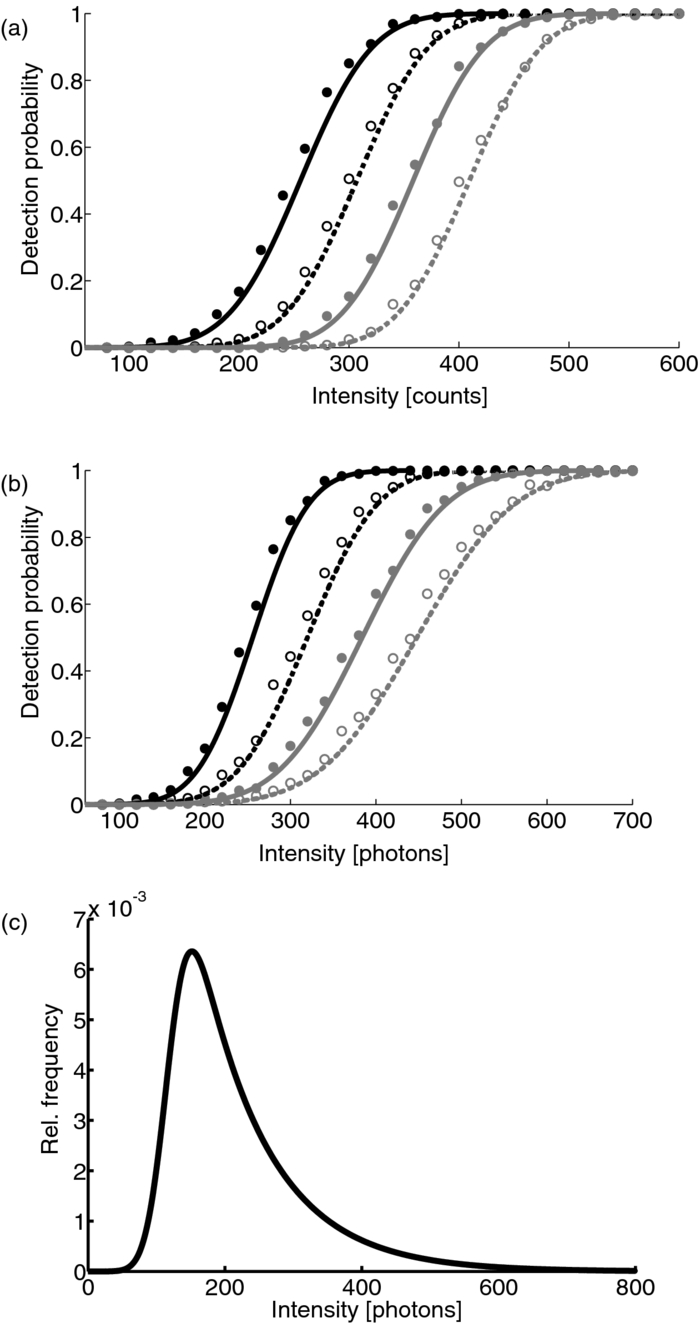

In experiments, the noise level σ is not constant but varies between images and, more strongly, between different cells. Therefore, the detection probability must be determined as the average over all acquired images using the noise levels in those images

Eq. 5

[TeX:] \documentclass[12pt]{minimal}\begin{document} \begin{equation} \overline{p_{\rm{det}}^{\mathrm{max}}}(S; w,t) = \frac{1}{N_{\rm{images}}}\sum _{i}^{N_{\rm{images}}} p_{\rm{det}}^{\mathrm{max}}(S; \sigma _{i},w,t), \end{equation} \end{document}

\bar{p_{\det}^{\max}} (S; w, t) = \frac{1}{N_{images}} \sum_{i}^{N_{images}} p_{\det}^{\max} (S; σ_{i}, w, t),

where σ_i is the noise level in image i and N _images is the number of acquired images.

With the help of [Eq. 5], we can now theoretically determine the shape of measured intensity distributions, which are products of the distribution of the emitted intensities [Eq. 1] and the detection probability [Eq. 5]. An example for the intensity distribution of a single fluorophore is given in Fig. 2c. Because the detection probability goes to 0 for small intensities, measured intensity distributions always have a peak at finite intensities, despite the fact that the underlying distribution of emitted intensities is maximal for small intensities. In Sec. 3, we will show that experimentally determined intensity distributions indeed have the predicted shape shown in Fig. 2c.

To find the optimal value for the threshold t, we must balance the number of rejected single-molecule signals, which increases with t, with the number of false positives (i.e., noise accepted as signal), which decreases with t. To predict the number of false positives, we calculated the probability p _false(t) to falsely detect a single molecule in a pixel with only noise at threshold t (see also Appendix xB),

Eq. 6

[TeX:] \documentclass[12pt]{minimal}\begin{document} \begin{equation} p_{\rm{false}}(t) = \frac{1}{2} \left[ 1 + \mathrm{erf}\left(- \frac{t}{\sqrt{2}} \right) \right] . \end{equation} \end{document}

p_{false} (t) = \frac{1}{2} [1 + \erf (- \frac{t}{\sqrt{2}})] .

In an image with M pixels, roughly Mp _false(t) noise peaks are falsely detected as single, molecule signals, if the pixels can be considered independent. We define ε as the maximal allowed ratio of false positives [Mp _false(t)] to all detected signals N _signals: Mp _false(t) < εN _signals. This definition leads to an upper limit for t,

Eq. 7

[TeX:] \documentclass[12pt]{minimal}\begin{document} \begin{equation} t > \sqrt{2} \; \mathrm{erf}^{-1} \left(1 - 2 \varepsilon \frac{N_{\rm{signals}}}{M}\right) . \end{equation} \end{document}

t > \sqrt{2} \erf^{- 1} (1 - 2 ɛ \frac{N_{signals}}{M}) .

For example with ε = 0.01, M = 50², and typically N _signals = 10, we get t ≳ 4. Because the total number of detected signals depends on N _signals and will decrease with t, t should not be chosen too large to avoid loss of data.

3. Experimental

3.1.

Deoxyribonucleics Acid Constructs

The protocol for the preparation of the deoxyribonucleics acid (DNA) constructs was previously described in detail in Ref. 15. The DNA sequence encoding the 10 C-terminal amino acids of human HRAS (GCMSCKCVLS), which includes the CAAX motif, was inserted in the frame at the C-terminus of the EYFP (S65G/S72A/T203Y) coding sequence. The integrity of the reading frame of the resulting EYFP-C10HRAS construct was verified by sequence analysis. For expression in mammalian cells, the complete coding sequence was cloned into the pcDNA3.1 vector (Invitrogen, Groningen, The Netherlands).

3.2.

Cell Culture

For all experiments, a Chinese hamster ovary (CHO) cell line (clone D3) was used. Cells were cultured in DMEM:F12 1:1 medium supplemented with streptomycin (100 μg/ml), penicillin (100 U/ml) and 10% newborn calf serum in a 7% CO₂ humidified atmosphere at 37°C. Cells were used for 25 − 30 passages and were transferred every four days. For microscopy, cells were cultured on cover glass slides (Assistent, Karl Hecht KG, Sondheim, Germany) and transfected with 250 ng DNA and 3 μl FUGENE HD (Roche Molecular Biochemicals, Indianapolis, Indiana) per glass slide (1 h incubation time). For a convenient expression level cells were used three to four days after transfection.

3.3.

Single-Molecule Microscopy

The experimental setup for single-molecule imaging has been described in detail previously.¹⁵ Briefly, the microscope (Axiovert 100; Zeiss, Oberkochen, Germany) was equipped with a 100x oil-immersion objective (NA = 1.4, Zeiss, Oberkochen, Germany). The samples were illuminated for T = 50 ms by an Ar⁺ laser (Spectra Physics, Mountain View, California, USA) at a wavelength of 514 nm. The illumination intensity was set to 3 ± 0.3 kW/cm². A circular diaphragm was introduced in the back focal plane of the tube lens to confine the illumination area. This results in a flat laser illumination profile. An appropriate filter combination (DCLP530, ET550/50 m, Chroma Technology, Brattleboro, Vermont) permitted the detection of individual fluorophores by a liquid-nitrogen–cooled slow-scan CCD camera system (Princeton Instruments, Trenton, New Jersey). The total detection efficiency of the imaging optics was η_o = 0.12. The time between consecutive images (time lag, Δt) was set to 254 ms. Typically, 4000–8000 images were obtained per cell. Hence, cells were discontinuously illuminated for a total duration of ∼5 min during the 30-min data-acquisition time. In accordance with earlier studies,^{3, 15} no signs of photodamage¹⁹ were observed after this illumination protocol.

For the observation of the intensity of individual EYFP-C10HRas, CHO cells adhered to glass slides were mounted onto the microscope and kept in phosphate-buffered saline [(PBS): 150 mM NaCl, 10 mM Na₂HPO₄/NaH₂PO₄, pH 7.4] at 37°C. The focus of the microscope was set to the bottom membrane of individual cells (depth of focus ≈1 μm). The density of fluorescent proteins on the plasma membrane of selected transfected cells was <1 μm⁻² to permit imaging of individual fluorophores.

According to Ref. 20 the bleaching time τ_bl for the used laser intensity I _ill = 3 kW/cm² is 10.4 ms. The probability that a single EYFP bleaches within the illumination/integration time T = 50 ms is therefore p _bl > 99%.²⁰ In other words, a single EYFP is bleached within the illumination time. The bleaching rate k _bl = 1/τ_bl is well separated from 1/T (k _bl ≈ 0.2T ⁻¹), and therefore, the simplified model described later [see Eq. 1] is applicable.

The expected photon emission rate expected from results in Ref. 20 is F = 775 photons/ms. Therefore, N = η_oτ_bl F ≈ 970 photons are expected to be detected during the average lifetime τ_bl of the fluorophore, where the detection efficiency is η_o = 0.12.

3.4.

Image Analysis

At first, the autofluorescent background is subtracted from the raw images. The background-subtracted images are subsequently filtered with a 2-D Gaussian whose width corresponds to the width of the PSF of the microscope. This procedure optimizes the signal-to-noise ratio. The positions of the pixels whose value after filtering exceeds a certain multiple of the noise are used as initial values for the fitting of a 2-D Gaussian in the unfiltered image. From this fit, position, width, and integrated intensity of the single-molecule signal are determined (see Fig. 3). Note that we define the standard deviation of the 2-D Gaussian as signal width w and not the FWHM. The width w is related to the FWHM of the signals¹⁸ by the relation [TeX:] \documentclass[12pt]{minimal}\begin{document}$w = \text{FWHM}/ \sqrt{8 \ln 2}$\end{document} $w = FWHM / \sqrt{8 \ln 2}$ . More details can be found Appendix xB.

Fig. 3

In vivo fluorescence imaging of EYFP-C10HRas; (a) Left: Fluorescence signals coming from single EYFP-C10HRas in a live cell. Right: 1-D example for peak fitting. A Gaussian (black line) is fitted to the raw data (red dots) to determine position, width and integrated signal intensity. Pixels = 220 nm. (b) Confocal scan of a group of CHO cells expressing EYFP-C10HRAS. (c) A montage of consecutive confocal slices shows that the protein is mainly found at the plasma membrane and the golgi apparatus. (d) and (e) TIRF image of a group of five CHO cells (denoted by roman numerals) expressing EYFP-C10HRAS at various levels. Image intensities are autoscaled with respect to cell I (d) or III (e). The signal density of cell III (0.24 μm⁻²) falls in the upper range of cells that have been selected for analysis. scale bars = 10 μm.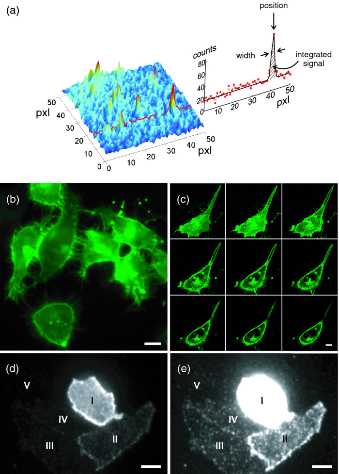

4. Results and Discussion

4.1.

Experimental Validation

To verify our theoretical derivations, we performed single-molecule fluorescence experiments on membrane-anchored EYFP (EYFP-C10HRas) in CHO cells. EYFP was tagged to the membrane-anchor of HRAS, which resulted in a membrane localization of EYFP-C10HRAS, as confirmed by confocal microscopy [Figs. 3b, 3c] and thereby greatly facilitated the measurements. We measured the intensities of ≈23 × 10³ diffraction-limited signals integrated over an illumination time of T = 50 ms. Estimations from earlier experiments (see Sec. 3) revealed that an illumination time of 50 ms is several times larger than the bleaching time expected at the illumination intensities used. In other words, single EYFP was bleached while being recorded. Attempts to track the movement of individual EYFP-C10HRAS failed, which further confirms that each EYFP was bleached within the illumination time.

A clear goal of this study was to perform all measurements in the context of living cells. Hence, intensity distribution of true monomeric EYFP molecules were not obtained from in vitro measurements on purified proteins.²⁰ Rather, we sought to obviate possible changes of the photophysical properties of EYFP, which could be introduced by an in vitro protocol involving protein extraction and immobilization of EYFP or EYFP-C10HRAS. Consequently, intensity distributions of monomeric EYFP were obtained from in vivo measurements on cells expressing EYFP-C10HRAS. To do this, we had to ensure that only a single EYFP-C10HRAS was present in each diffraction-limited spot. To meet this requirement, the density of EYFP-C10HRAS was kept very low (≈0.2 μm⁻²), which was achieved by first selecting cells with very low expression levels [Figs. 3d, 3e] followed by a deep photobleaching of the whole cell body.

Of note, this protocol can be readily applied to a wide variety of similar scenarios. Every protein, which may participate in a process involving dimer or cluster formation can be assessed (i) in its resting stage, (ii) at low expression levels, and (iii) after intense photobleaching to obtain an intensity distribution of the attached fluorophore for the true or close to monomeric status of the protein.

Figure 4a shows the obtained intensity distribution. We used a threshold factor of t = 3 and plotted only signal intensities >1000 photons, where the influence of the detection probability on the distribution is negligible. Also, the number of false positives due to noise is minimized in this way. As expected from theory [Eq. 1] the distribution approximately follows an exponential decay. The measured mean number of photons of N = 837 ± 3 is in agreement with the value expected from earlier results on EYFP (N = 970; Sec. 3).

To demonstrate the influence of thresholding on intensity distributions, we present in Fig. 4b several intensity distributions based on the same raw data, which differ by the threshold factor t. In principle, these distributions should be the product of the distribution of emitted photons [Eq. 1], with the mean number of photons N determined above [see Fig. 4a], and the detection probability at a certain threshold factor t and noise level σ. This product is given in [Eq. 31]. The noise levels were estimated as described in Appendix xB. The resulting detection probability [TeX:] \documentclass[12pt]{minimal}\begin{document}$\overline{p_{\rm{det}}^{\mathrm{max}}}(S;w,t)$\end{document} $\bar{p_{\det}^{\max}} (S; w, t)$ is then multiplied with the distribution of emitted intensities [Eq. 1] to get the full theoretical description of the measured intensity distributions [solid lines in Fig. 4b]. The measured distributions precisely follow the theoretical expressions determined in this way. The limitations of our approach are discussed in Appendix xD.

4.2.

Clustering Due to Membrane Heterogeneity

The measurements presented in the Sec. 4.1 were performed at low expression levels to ensure the presence of only a single EYFP-C10HRAS per diffraction-limited spot. In subsequent measurements at increased densities of EYFP-C10HRAS, we observed a shift of the intensity distributions toward higher intensities (see Fig. 5). This shift is due to the presence of several molecules in one diffraction-limited spot. Without creating the view of molecular interaction, we will refer to two or more labeled proteins per spot as a dimer or cluster, respectively.

Fig. 4

Intensity distribution of single EYFP-C10HRAS in the membrane of living CHO cells. (a) Experimental intensity distribution of the intensities of 22,615 single-molecule fluorescence signals (solid circles). A one-parameter fit of [Eq. 1] (solid line) to the experimental intensity distribution for single EYFP-C10HRAS gives N = 837 ± 3 photons. The width w of the single-molecule signals was restricted to the interval 0.64 − 0.81 pixel, the width of the 2-D Gaussian filter was r = 0.72 pixels, pixels = 220 nm. The threshold factor was t = 3, and only signals with an intensity of 1000 photons were used. (b) Influence of thresholding on the shape of the intensity distributions. The raw data are the same as in (a), but the threshold factor t is varied, t = 5, 10, 15, 20. The experimental data (solid circles) a compared to the full theoretical distribution [Eq. 31] (solid line). The mean number of detected photons N was determined above from a restricted data set [see (a)]; the detection probability was calculated by integration over the noise levels found in the raw images.

Fig. 5

Influence of membrane heterogeneity on the intensity distribution of EYFP-C10HRAS in the membrane of living CHO cells. The solid circles give the intensity distribution at low signal densities (<0.2 μm⁻²), already shown in Fig. 4. The solid line is the corresponding theoretically expected distribution obtained as detailed earlier. This distribution is compared to one taken at a signal density of 0.25 μm⁻² (open circles). The threshold factor is t = 3 for both distributions. The visible shift to higher intensities with increased signal densities is due to the presence of multimers (i.e., several molecules colocalized in a diffraction limited spot). A fit to [Eq. 8] (dashed line) gives that at this density the fraction of monomers is α = 0.14. Inset: Fraction of monomers versus density of single molecule signals (solid circles). The error was determined as standard deviation calculated from all data sets used in a certain bin. The open circles show the theoretically expected monomer fraction for a uniform distribution of molecules, [see Eq. 34].

To quantify the amounts of monomers, dimers, and higher multimers, we compare the intensity distributions at various densities of single-molecule signals to the intensity distribution of the monomer.¹⁰ For simplicity, we assume here that only monomers and dimers are present and describe the measured distributions as a weighted sum of the intensity distribution of a monomer p(n; N) and a dimer p ₂(n; N)

Eq. 8

[TeX:] \documentclass[12pt]{minimal}\begin{document} \begin{equation} p_{\rm{total}}(n) = \alpha \, p(n;N) + (1-\alpha) \, p_{2}(n;N). \end{equation} \end{document}

p_{total} (n) = α p (n; N) + (1 - α) p_{2} (n; N) .

p(n; N) and p ₂(n; N) were presented above in Sec. 2.2 (see Appendix xA, for the derivation). N, the average number of detected photons, is determined from the monomer distribution as described in Sec. 4.1, which leaves the fraction of monomers α as the sole fit parameter. Figure 5 shows an example for a fit of this model to experimental data. We find that α decreases quickly with increasing signal density (see inset of Fig. 5). The error for the determination of α is discussed in Appendix xD.

Strikingly, there are many more dimers than one would expected for a uniform distribution of molecules at such low densities (<1 μm⁻²; see model derived in Appendix xC). This finding is in agreement with earlier results on the used construct,¹⁵ where a certain fraction of these molecules was shown to exhibit confined diffusion in ≈200 nm domains. Thus, for the distribution of the membrane anchor HRAS, colocalization of molecules even at low densities, is expected.

5. Conclusion

We have shown that our method is able to employ fluorescence intensity as a faithful readout of membrane heterogeneity related clustering. The accurate and quantitative description of the intensity distribution of EYFP-fusion proteins in vivo allows us to characterize the spatial distribution of membrane proteins, which may be based on membrane heterogeneities or domain formations on the length scale of or below the diffraction limit. Although, inherently, the method is not able to report the exact size of such domains, it makes up for this lack of spatial resolution by providing temporal resolution. With our method, the status of domain presence, can in principle, be monitored repeatedly (i.e., many times in the course of a biological reaction, such as a signaling event).

The technique is similar to PCHs,²¹ in the sense that we measure photon emission from single molecules. However, although PCH measurments use illumination times that are chosen as short as possible to be able to resolve intensity fluctuations, our method employs the opposite limit: we choose the illumination time such that the measured photon count does not depend on the time of measurement. Although PCH is perfectly able to retrieve stochiometries, our method has the advantage that we do not have to measure the photon emission from a molecule several times to build a histogram but extract all necessary information in one shot. Hence, our method is better suited to follow changes in stoichiometry, e.g., the formation of true protein complexes (i.e., molecular dimers, trimers, or higher multimers), as this would also lead to intensity distributions, from which our method could extract thestoichiometry and its changes. However, as our results show, membrane heterogeneity must be taken into account when true complex formation is to be measured.

Appendices

Appendix A: Intensity Distribution

Mandel Theory

According to the semiclassical theory by Mandel,¹⁴ which is used also in PCHs,²¹ the probability to find n photons at time t with an integration/illumination time T and detector quantum yield η_d is

Eq. 9

[TeX:] \documentclass[12pt]{minimal}\begin{document} \begin{eqnarray} p(n,t,T) &=& \int _{0}^{\infty } \frac{\left(\eta _{\rm d} W(t)\right)^{n} e^{-\eta _{\rm d} W(t)}}{n!} p_{\rm{inc}}[W(t),T] dW(t),\nonumber \\ W(t) &=& \eta _{\rm o} \int _{t}^{T+t} \int _{\rm A} I(\mathbf {r},t) d \mathbf {A} dt . \end{eqnarray} \end{document}

\begin{matrix} p (n, t, T) & = & \int_{0}^{\infty} \frac{{(η_{d} W (t))}^{n} e^{- η_{d} W (t)}}{n!} p_{inc} [W (t), T] d W (t), \\ W (t) & = & η_{o} \int_{t}^{T + t} \int_{A} I (r, t) d A d t . \end{matrix}

W(t) is the number of incident photons falling on the detector given a photon emission rate [TeX:] \documentclass[12pt]{minimal}\begin{document}$I(\mathbf {r},t)$\end{document}

I (r, t)

, a detection efficiency of the imaging optics η_o and a detector area A. p _inc[W(t), T] is the probability distribution of the number of incident photons W(t) at time t given an illumination time T.

Here integration is performed not over the whole detector (which would be the whole CCD chip) but over the area on the chip that is covered by a single-molecule signal so that

Eq. 10

[TeX:] \documentclass[12pt]{minimal}\begin{document} \begin{equation} W(t) = \eta _{\rm o} \int _{t}^{T+t} I_{\rm{sm}}(t) dt ,\end{equation} \end{document}

W (t) = η_{o} \int_{t}^{T + t} I_{sm} (t) d t,

where I _sm(t) is the photon emission rate coming from a single molecule. T is assumed to be so long that W(t) is independent of the time of measurement t: W(t) ≡ W. Note that this is the opposite of the limit used in PCH,²¹ where very short integration/illumination times T are used so that the intensity fluctuations govern the counting statistics. For long, enough illumination times T the probability distribution p _inc(W, T) can be obtained from the probability p _fluor(t _on, T) that a molecule is “on”, (i.e., emitting photons, for a period t _on during the integration time T). If [TeX:] \documentclass[12pt]{minimal}\begin{document}$\bar{I}$\end{document}

\bar{I}

is the average number of photons emitted during periods when the molecule is on, p _inc(W, T) is

Eq. 11

[TeX:] \documentclass[12pt]{minimal}\begin{document} \begin{equation} p_{\rm{inc}}(W,T) = \frac{1}{\eta _{\rm o}\bar{I}} \; p_{\rm{fluor}}\left(t_{\rm{on}} = \frac{W}{\eta _{\rm o} \bar{I}},T \right) .\end{equation} \end{document}

p_{inc} (W, T) = \frac{1}{η_{o} \bar{I}} p_{fluor} (t_{on} = \frac{W}{η_{o} \bar{I}}, T) .

The distribution of the on times, p _fluor(t _on, T), depends on the photophysics of the molecule. In the following two paragraphs a model for p _fluor(t _on, T) that includes blinking and bleaching is derived.

Two-State Model

The two-state model with a fluorescent on and a non-fluorescent off state was discussed in Ref. 22. In this model, the molecule can switch reversibly between the on and the off states, but it never bleaches. The corresponding probability distribution for the times t _on in the on state p _fluor(t _on, T) is the sum of contributions from four different kinds of fluorescence traces: (i) A molecule that starts in the on state can stay on during the whole illumination time T (t _on = T). The probability for such a trace is p _on(0)exp (− k _off T) where p _on(0) is the probability that the molecule is initially on and k _off is the rate for switching from on to off. (ii) A molecule that starts in the off state can stay off during the whole illumination time T (t _on = 0) . The probability for such a trace is p _off(0)exp (− k _on T), where p _off(0) is the probability that the molecule is initially off and k _on is the rate for switching from off to on. Because a molecule can either be on or off initially, p _on(0) + p _off(0) = 1 must hold. (iii). A molecule that starts in the on state can switch between on and off. The probability density for those fluorescence traces is

Eq. 12

[TeX:] \documentclass[12pt]{minimal}\begin{document} \begin{eqnarray} p_{\rm{odd}} (t_{\rm{on}},T) &=& k_{\rm{off}} \exp \left(-k_{\rm{off}}t_{\rm{on}} - k_{\rm{on}}t_{\rm{off}} \right) \\ & &\times\, I_{0} (2\sqrt{k_{\rm{off}}k_{\rm{on}}t_{\rm{on}}t_{\rm{off}}}), \nonumber \end{eqnarray} \end{document}

\begin{matrix} p_{odd} (t_{on}, T) & = & k_{off} \exp (- k_{off} t_{on} - k_{on} t_{off}) \\ \times I_{0} (2 \sqrt{k_{off} k_{on} t_{on} t_{off}}), \end{matrix}

for an odd number of switches and

Eq. 13

[TeX:] \documentclass[12pt]{minimal}\begin{document} \begin{eqnarray} p_{\rm{even}} (t_{\rm{on}},T) &=& \sqrt{k_{\rm{off}}k_{\rm{on}}\frac{t_{\rm{on}}}{t_{\rm{off}}} } \exp \left(-k_{\rm{off}}t_{\rm{on}} - k_{\rm{on}}t_{\rm{off}} \right) \nonumber \\ &&\times\, I_{1} (2\sqrt{k_{\rm{off}}k_{\rm{on}}t_{\rm{on}}t_{\rm{off}}}), \end{eqnarray} \end{document}

\begin{matrix} p_{even} (t_{on}, T) & = & \sqrt{k_{off} k_{on} \frac{t_{on}}{t_{off}}} \exp (- k_{off} t_{on} - k_{on} t_{off}) \\ \times I_{1} (2 \sqrt{k_{off} k_{on} t_{on} t_{off}}), \end{matrix}

for an even number of switches. t _off = T − t _on, and I ₀ and I ₁ are modified Bessel functions of the first kind of order 0 and 1, respectively (see Ref. 22). The total probability for traces that start in the on state and switch between on and off is p _on(0)[p _odd(t _on, T) + p _even(t _on, T)]. (iv) The probability density for a molecule that starts in the off state and switches between off and on are analogous: k _on is interchanged with k _off and t _on is interchanged with t _off.

The total probability density for the on times t _on is the sum of all four contributions

Eq. 14

[TeX:] \documentclass[12pt]{minimal}\begin{document} \begin{eqnarray} p_{\rm{fluor}}(t_{\rm{on}},T) &=& p_{\rm{on}}(0)\exp (-k_{\rm{off}}T) \delta (T - t_{\rm{on}}) + p_{\rm{off}}(0)\nonumber\\ && \times\, \exp (-k_{\rm{on}}T)\delta (t_{\rm{on}}) + \Theta (t_{\rm{on}})\Theta (T-t_{\rm{on}}) \nonumber \\ && \times \exp (-k_{\rm{off}}t_{\rm{on}} - k_{\rm{on}}t_{\rm{off}}) [ (p_{\rm{on}}(0) k_{\rm{off}}\nonumber\\ && +\, p_{\rm{off}}(0)k_{\rm{on}}) I_{0} (2\sqrt{k_{\rm{off}}k_{\rm{on}}t_{\rm{on}}t_{\rm{off}}}) \nonumber \\ && + (p_{\rm{on}}(0) \sqrt{t_{\rm{on}}/t_{\rm{off}}} +\! p_{\rm{off}}(0)\sqrt{t_{\rm{off}}/t_{\rm{on}}}) \sqrt{k_{\rm{off}}k_{\rm{on}}} I_{1} \nonumber\\ && \times\, (2\sqrt{k_{\rm{off}}k_{\rm{on}}t_{\rm{on}}t_{\rm{off}}}) ] .\!\!\! \end{eqnarray} \end{document}

\begin{matrix} p_{fluor} (t_{on}, T) & = & p_{on} (0) \exp (- k_{off} T) δ (T - t_{on}) + p_{off} (0) \\ \times \exp (- k_{on} T) δ (t_{on}) + Θ (t_{on}) Θ (T - t_{on}) \\ \times \exp (- k_{off} t_{on} - k_{on} t_{off}) [(p_{on} (0) k_{off} \\ + p_{off} (0) k_{on}) I_{0} (2 \sqrt{k_{off} k_{on} t_{on} t_{off}}) \\ + (p_{on} (0) \sqrt{t_{on} / t_{off}} + p_{off} (0) \sqrt{t_{off} / t_{on}}) \sqrt{k_{off} k_{on}} I_{1} \\ \times (2 \sqrt{k_{off} k_{on} t_{on} t_{off}})] . \end{matrix}

Three-State Model

We generalize the above model presented in Sec. A.2 to a three-state model in which the fluorophore can bleach from the on state to a bleached state with rate k _bl [see inset to Fig. 1a]. In this model, the probability distribution p _fluor(t _on, T) is again given by the sum of four contributions. (i) A molecule starts in the on state and stays on during the whole illumination time T (t _on = T). The probability for such traces is now p _on(0)exp [ − (k _off + k _bl)T]. (ii) The probability that the molecule starts in the off state and stays off during T (t _on = 0) is as above: p _off(0)exp (− k _on T). (iii) The contribution of traces that are switching and end in the on or off state without bleaching during the illumination time T is the same as contribution (iii) of the two-state model except for an additional factor exp (− k _bl t _on). (iv) A molecule can start in the on or off, state, and after several switching events, the fluorescence trace is ended by a final bleaching event from the on state. The probability that a molecule is initially on and stays on until it bleaches at time t _on is p _on(0)k _blexp [ − (k _bl + k _off)t _on]. If the molecule switches, then it must switch an even number of times if it is initially on, and an odd number of times if it is initially off to end the fluorescence trace in the on state before bleaching. The corresponding probabilities are p _on(0)p _even(t _on, t′) and p _off(0)p _odd(t _on, t′) where t′ is the point in time when the bleaching event takes place. t′ lies between t _on (then the molecule is continuously on until it bleaches) and T (then t _on is spread over the illumination time T) (see Fig. 6).

Fig. 6

Illustration of fluorescence traces contributing to the probability distribution p _fluor(t _on, T). In all three cases, the on time is identical while the time point of bleaching t′ is varied. In the topmost trace, the time of bleaching t′ is identical to t _on, the molecule must be continuously in the on state until bleaching. In the middle trace, the on time is spread over the time until bleaching due to intermittent periods in the off state. In the bottom trace, the molecule bleaches exactly at the end of the illumination period. The on time is spread over the whole illumination period T.

To properly account for all possible traces, one has to integrate t′ over all allowed values t _on < t′ < T. Finally, the probability for a bleaching event after an on time of t _on is k _blexp (− k _bl t _on). In summary, the contribution of switching traces that are ended by a final bleaching event is

Eq. 15

[TeX:] \documentclass[12pt]{minimal}\begin{document} \begin{eqnarray} &&\hspace*{-1pc} p_{\rm{on}}(0) k_{\rm{bl}}\exp [-(k_{\rm{bl}}+k_{\rm{off}})t_{\rm{on}}] + k_{\rm{bl}}\exp (-k_{\rm{bl}}t_{\rm{on}}) \nonumber \\ && \times\, \int _{t_{\rm{on}}}^{T}dt^{\prime }[p_{\rm{on}}(0)p_{\rm{even}}(t_{\rm{on}},t^{\prime }) + p_{\rm{off}}(0)p_{\rm{odd}}(t_{\rm{on}},t^{\prime }) ].\quad \end{eqnarray} \end{document}

\begin{matrix} p_{on} (0) k_{bl} \exp [- (k_{bl} + k_{off}) t_{on}] + k_{bl} \exp (- k_{bl} t_{on}) \\ \times \int_{t_{on}}^{T} d t^{'} [p_{on} (0) p_{even} (t_{on}, t^{'}) + p_{off} (0) p_{odd} (t_{on}, t^{'})] . \end{matrix}

Adding the contributions from the four different kinds of fluorescence traces results in

Eq. 16

[TeX:] \documentclass[12pt]{minimal}\begin{document} \begin{eqnarray} \nonumber\\[-3pc] p_{\rm{fluor}}(t_{\rm{on}},T) &=& p_{\rm{on}}(0) \exp \left[-(k_{\rm{off}} + k_{\rm{bl}})T\right] \delta (T-t_{\rm{on}}) + p_{\rm{off}}(0) \exp (-k_{\rm{on}}T)\delta (t_{\rm{on}}) + \Theta (t_{\rm{on}})\Theta (T-t_{\rm{on}}) \nonumber \\ &&\times \left(k_{\rm{bl}}\exp (-k_{\rm{bl}}t_{\rm{on}}) \left[p_{\rm{on}}(0)\exp (-k_{\rm{off}}t_{\rm{on}}) + \int _{t_{\rm{on}}}^{T}dt^{\prime }[p_{\rm{on}}(0)p_{\rm{even}}(t_{\rm{on}};t^{\prime }) + p_{\rm{off}}(0)p_{\rm{odd}}(t_{\rm{on}};t^{\prime }) ] \right] \right.\nonumber \\ && + \exp (-k_{\rm{bl}}t_{\rm{on}}) \exp (-k_{\rm{off}}t_{\rm{on}} - k_{\rm{on}}t_{\rm{off}}) \{ [p_{\rm{on}}(0) k_{\rm{off}} + p_{\rm{off}}(0)k_{\rm{on}}] I_{0} (2\sqrt{k_{\rm{off}}k_{\rm{on}}t_{\rm{on}}t_{\rm{off}}}) \nonumber \\ && \left. +\, [p_{\rm{on}}(0) \sqrt{t_{\rm{on}}/t_{\rm{off}}} + p_{\rm{off}}(0)\sqrt{t_{\rm{off}}/t_{\rm{on}}}] \sqrt{k_{\rm{off}}k_{\rm{on}}} I_{1} (2\sqrt{k_{\rm{off}}k_{\rm{on}}t_{\rm{on}}t_{\rm{off}}}) \} \right) . \end{eqnarray} \end{document}

\begin{matrix} p_{fluor} (t_{on}, T) & = & p_{on} (0) \exp [- (k_{off} + k_{bl}) T] δ (T - t_{on}) + p_{off} (0) \exp (- k_{on} T) δ (t_{on}) + Θ (t_{on}) Θ (T - t_{on}) \\ \times (k_{bl} \exp (- k_{bl} t_{on}) [p_{on} (0) \exp (- k_{off} t_{on}) + \int_{t_{on}}^{T} d t^{'} [p_{on} (0) p_{even} (t_{on}; t^{'}) + p_{off} (0) p_{odd} (t_{on}; t^{'})]] \\ + \exp (- k_{bl} t_{on}) \exp (- k_{off} t_{on} - k_{on} t_{off}) {[p_{on} (0) k_{off} + p_{off} (0) k_{on}] I_{0} (2 \sqrt{k_{off} k_{on} t_{on} t_{off}}) \\ + [p_{on} (0) \sqrt{t_{on} / t_{off}} + p_{off} (0) \sqrt{t_{off} / t_{on}}] \sqrt{k_{off} k_{on}} I_{1} (2 \sqrt{k_{off} k_{on} t_{on} t_{off}})}) . \end{matrix}

We simplify this model by assuming that on and off rates are equal (k _on = k _off = k) and that the molecule is initially always in the on state [p _on(0) = 1, p _off(0) = 0].

If we use the probability distribution p _fluor(t _on, T) for the three-state model [Eq. 16] to calculate the distribution of incident photons p _inc(W, T) [Eq. 11] and insert p _inc(W, T) in Mandel's theory [Eq. 9], then we obtain the probability distribution p(n, T) for the number of photons detected during illumination time T. This distribution was used to illustrate the influence of blinking and bleaching in the Sec. 2.1.

Robust Intensity Distributions

If the illumination time T is so big that bleaching is fast on the time scale set by T (k _bl > 1/T), then the molecule bleaches within the illumination time T. If, additionally, blinking is faster than bleaching k > k _bl, then the molecule switches frequently between the on and off states during 1/k _bl and k _bl is the only relevant rate. Under these conditions, we can significantly simplify [Eq. 16] to

Eq. 17

[TeX:] \documentclass[12pt]{minimal}\begin{document} \begin{eqnarray} p_{\rm{fluor}}(t_{\rm{on}}) &=& k_{\rm{bl}} \exp \left(-k_{\rm{bl}}t_{\rm{on}} \right) \nonumber \\ \Rightarrow p_{\rm{inc}}(W) &=& \frac{k_{\rm{bl}}}{\eta _{\rm o} \bar{I}} \exp \left(-\frac{k_{\rm{bl}}W}{\eta _{\rm o}\bar{I}} \right) . \end{eqnarray} \end{document}

\begin{matrix} p_{fluor} (t_{on}) & = & k_{bl} \exp (- k_{bl} t_{on}) \\ \Rightarrow p_{inc} (W) & = & \frac{k_{bl}}{η_{o} \bar{I}} \exp (- \frac{k_{bl} W}{η_{o} \bar{I}}) . \end{matrix}

If we insert this distribution into Mandel's formula [Eq. 9] then we get

Eq. 18

[TeX:] \documentclass[12pt]{minimal}\begin{document} {\fontsize{8.5}{9.5}{\begin{eqnarray} p(n,T) \equiv p(n) &=& \int _{0}^{\infty } \frac{\left(\eta _{\rm d} W\right)^{n} e^{-\eta _{\rm d} W}}{n!} \cdot \frac{k_{\rm{bl}}}{\eta _{\rm o}\bar{I} } \exp \left(-\frac{k_{\rm{bl}}W}{\eta _{\rm o}\bar{I} } \right) dW \nonumber \\ &=& \frac{k_{\rm{bl}}}{ \eta _{\rm o}\bar{I} } \frac{\eta _{\rm d}^{n}}{n!} \int _{0}^{\infty } W^{n} e^{- \eta W} dW \quad \rm{with} \quad \eta = \eta _{\rm d} + \frac{k_{\rm{bl}}}{\eta _{\rm o}\bar{I} } \nonumber \\ &=& \! \frac{ k_{\rm{bl}}}{\eta _{\rm o}\bar{I} } \eta _{\rm d}^{n}\eta ^{-(n+1)} {=} \frac{1}{1 + \eta _{\rm d} \eta _{\rm o} \bar{I}k_{\rm{bl}}^{-1} } \left(1 \,{+}\, \frac{1}{\eta _{\rm d} \eta _{\rm o} \bar{I} } k_{\rm{bl}}^{-1} \right)^{-n}\!\!\!.\nonumber \!\!\!\! \\ \end{eqnarray}}} \end{document}

\begin{matrix} p (n, T) \equiv p (n) & = & \int_{0}^{\infty} \frac{{(η_{d} W)}^{n} e^{- η_{d} W}}{n!} \cdot \frac{k_{bl}}{η_{o} \bar{I}} \exp (- \frac{k_{bl} W}{η_{o} \bar{I}}) d W \\ = & \frac{k_{bl}}{η_{o} \bar{I}} \frac{η_{d}^{n}}{n!} \int_{0}^{\infty} W^{n} e^{- η W} d W with η = η_{d} + \frac{k_{bl}}{η_{o} \bar{I}} \\ = & \frac{k_{bl}}{η_{o} \bar{I}} η_{d}^{n} η^{- (n + 1)} = \frac{1}{1 + η_{d} η_{o} \bar{I} k_{bl}^{- 1}} {(1 + \frac{1}{η_{d} η_{o} \bar{I}} k_{bl}^{- 1})}^{- n} . \end{matrix}

By introducing [TeX:] \documentclass[12pt]{minimal}\begin{document}$N = \eta _{\rm d} \eta _{\rm o} \bar{I} k_{\rm{bl}}^{-1}$\end{document}

N = η_{d} η_{o} \bar{I} k_{bl}^{- 1}

we can write this distribution for the number of detected photons n as

Eq. 19

[TeX:] \documentclass[12pt]{minimal}\begin{document} \begin{equation} p(n;N)= \frac{1}{N} \left(1 + \frac{1}{N}\right)^{-(n+1)}, \end{equation} \end{document}

p (n; N) = \frac{1}{N} {(1 + \frac{1}{N})}^{- (n + 1)},

where N is the average number of photons detected [TeX:] \documentclass[12pt]{minimal}\begin{document}$N = \sum _{n=0}^{\infty } n \, p(n)$\end{document}

N = \sum_{n = 0}^{\infty} n p (n)

.

In order to estimate the range of parameters in which the simplified model is valid, we compare it to the full model [Eq. 16]. Figure 7 shows that the model works best, if k _bl is well separated from the blinking rates k and 1/T. As mentioned in Sec. 3 and in Appendix xD, this is indeed the case for the used experimental parameters.

Fig. 7

Comparison of the general model based on [Eq. 16] to the simplified model [Eq. 19] for long illumination times T. The open symbols correspond to the intensities calculated using the general model based on [Eq. 16] with bleaching rate k _bl = (0.05T)⁻¹ (open circles), k _bl = (0.1T)⁻¹ (open squares), and k _bl = (0.2T)⁻¹ (open triangles). The switching rate is k = (0.01T)⁻¹ for all distributions. The lines correspond to intensities given by [Eq. 19] with the same values for k _bl: k _bl = (0.05T)⁻¹ (black solid line), k _bl = (0.1T)⁻¹ (black dashed line), and k _bl = (0.2T)⁻¹ (gray solid line).

The distribution of the intensity of a dimer (i.e., two fluorophores in a diffraction-limited spot) p ₂(n; N) is obtained from the convolution of [Eq. 19] with itself,¹⁰

Eq. 20

[TeX:] \documentclass[12pt]{minimal}\begin{document} {\fontsize{9}{10}{\begin{eqnarray} p_{2}(n;N) &=& \sum _{n^{\prime }=0}^{\infty } p(n-n^{\prime })p(n^{\prime }) \nonumber \\ &&\hspace*{-25pt}= \frac{1}{(1 + N)^{2}} \sum _{n^{\prime } = 0}^{\infty } \left(1 + \frac{1}{N}\right)^{-(n-n^{\prime })} \Theta (n-n^{\prime }) \left(1 + \frac{1}{N}\right)^{-n^{\prime }}\hspace*{8pt} \nonumber \\ &&\hspace*{-25pt}= \frac{1}{(1 + N)^{2}} \left(1 + \frac{1}{N}\right)^{-n} \sum _{n^{\prime } = 0}^{n} = \frac{n+1}{(1 + N)^{2}} \left(1 + \frac{1}{N}\right)^{-n}. \hspace*{-28pt}\nonumber \\ \end{eqnarray}}} \end{document}

\begin{matrix} p_{2} (n; N) & = & \sum_{n^{'} = 0}^{\infty} p (n - n^{'}) p (n^{'}) \\ = \frac{1}{{(1 + N)}^{2}} \sum_{n^{'} = 0}^{\infty} {(1 + \frac{1}{N})}^{- (n - n^{'})} Θ (n - n^{'}) {(1 + \frac{1}{N})}^{- n^{'}} \\ = \frac{1}{{(1 + N)}^{2}} {(1 + \frac{1}{N})}^{- n} \sum_{n^{'} = 0}^{n} = \frac{n + 1}{{(1 + N)}^{2}} {(1 + \frac{1}{N})}^{- n} . \end{matrix}

Continued convolution with p(n; N)) [Eq.19] gives the distribution for higher multimers (e.g., a trimer),

Eq. 21

[TeX:] \documentclass[12pt]{minimal}\begin{document} \begin{eqnarray} p_{3}(n;N) &=& \sum _{n^{\prime }=0}^{\infty } p(n-n^{\prime })p_{2}(n^{\prime }) \nonumber \\ &=& \frac{1}{(1 + N)^{3}} \left(1 + \frac{1}{N}\right)^{-n} \sum _{n^{\prime } = 0}^{n} (n^{\prime }+1) \nonumber \\ &=& \frac{\left(n+1 \right)\left((n/2)+1 \right) }{(1 + N)^{3}} \left(1 + \frac{1}{N}\right)^{-n}. \end{eqnarray} \end{document}

\begin{matrix} p_{3} (n; N) & = & \sum_{n^{'} = 0}^{\infty} p (n - n^{'}) p_{2} (n^{'}) \\ = & \frac{1}{{(1 + N)}^{3}} {(1 + \frac{1}{N})}^{- n} \sum_{n^{'} = 0}^{n} (n^{'} + 1) \\ = & \frac{(n + 1) ((n / 2) + 1)}{{(1 + N)}^{3}} {(1 + \frac{1}{N})}^{- n} . \end{matrix}

In Fig. 1c gives the intensity distributions for a monomer, dimer, and trimer, with the same average number of detected photons N (per fluorophore) are compared.

Appendix B: Detection Probability

The fluorescence signal from a single molecule at position [TeX:] \documentclass[12pt]{minimal}\begin{document}$(\tilde{x},\tilde{y})$\end{document} $(\tilde{x}, \tilde{y})$ is given by the PSF of the microscope. The PSF, which is ideally a 2-D Airy function, is most commonly approximated by a 2-D Gaussian

Eq. 22

[TeX:] \documentclass[12pt]{minimal}\begin{document} \begin{equation} g(x,y) = \frac{S}{2 \pi w^2}\, \exp \left[ \frac{\left(x - \tilde{x}\right)^2 + \left(y - \tilde{y}\right)^2 }{2w^2} \right], \end{equation} \end{document}

g (x, y) = \frac{S}{2 π w^{2}} \exp [\frac{{(x - \tilde{x})}^{2} + {(y - \tilde{y})}^{2}}{2 w^{2}}],

where w is the width of the signal. Empirically, we find that, after background subtraction, the noise in the raw image is distributed normally with mean 0 and standard distribution σ (= noise level). The noise level can be estimated from the power spectral density (PSD) of the image. Because the noise is white, the average PSD for frequencies larger than 2/w equals σ².

To optimize the SNR, the image is filtered with an appropriate filter. According to optimal filtering theory,²³ the filter should be identical to the signal. Therefore, we filter with a 2-D Gaussian of width r. The resulting SNR is

Eq. 23

[TeX:] \documentclass[12pt]{minimal}\begin{document} \begin{equation} \mathrm{SNR} = \frac{Sr}{\sigma \sqrt{\pi } (r^2 + w^2) }, \end{equation} \end{document}

SNR = \frac{S r}{σ \sqrt{π} (r^{2} + w^{2})},

where [TeX:] \documentclass[12pt]{minimal}\begin{document}$\tilde{S} = S / [2 \pi (r^2 + w^2)]$\end{document}

\tilde{S} = S / [2 π (r^{2} + w^{2})]

is the maximum of the signal (= signal height) after filtering and [TeX:] \documentclass[12pt]{minimal}\begin{document}$\tilde{\sigma } = (\sigma /2 \sqrt{\pi }r)$\end{document}

\tilde{σ} = (σ / 2 \sqrt{π} r)

is the noise level after filtering. The noise distribution is still normal (with mean 0 and standard deviation [TeX:] \documentclass[12pt]{minimal}\begin{document}$\tilde{\sigma }$\end{document}

\tilde{σ}

). For the optimal choice r = w,

Eq. 24

[TeX:] \documentclass[12pt]{minimal}\begin{document} \begin{equation} \mathrm{SNR}_{\rm{max}} = \frac{S}{\sigma \sqrt{\pi }w } . \end{equation} \end{document}

{SNR}_{\max} = \frac{S}{σ \sqrt{π} w} .

Note that σ is in units of counts/pixel so that the SNR is dimensionless. In order to distinguish between noise and signal, a threshold t is introduced. Only those pixels in the filtered image whose brightness I(x, y) exceeds the (filtered) noise level by a factor t are treated as potential molecule positions,

Eq. 25

[TeX:] \documentclass[12pt]{minimal}\begin{document} \begin{equation} I(x,y) > t\, \frac{\sigma }{2 \sqrt{\pi }r} \equiv t \tilde{\sigma }. \end{equation} \end{document}

I (x, y) > t \frac{σ}{2 \sqrt{π} r} \equiv t \tilde{σ} .

Figure 8 illustrates the thresholding procedure.

Fig. 8

Thresholding procedure; (a) Raw image of single EYFP-C10HRas in the membrane of a living CHO cell. The noise is approximately σ = 26. The linear gray scale ranges from 0 counts (black) to 1002 counts (white). (b) Image after background subtraction and filtering (i.e., correlation) with 2-D Gaussian of width 0.7 pixels, pixels = 220 nm. The linear gray scale ranges from 0 counts (black) to 1473 counts (white). (c) Binary image after thresholding. White pixels correspond to pixels whose value exceeds the threshold at threshold factor t = 10.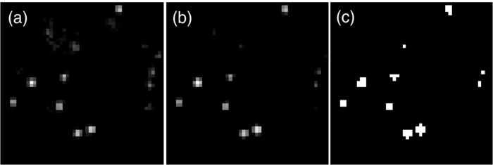

Subimages of the unfiltered image around the that which were identified as potential molecule positions are then fit with the sum of a 2-D Gaussian and a constant offset g(x, y) + off.

We define the detection probability p _det(σ, S) as the probability that, for a given noise level σ, a pixel with brightness [TeX:] \documentclass[12pt]{minimal}\begin{document}$\tilde{S}$\end{document} $\tilde{S}$ exceeds the threshold described; thus,

Eq. 26

[TeX:] \documentclass[12pt]{minimal}\begin{document} \begin{equation} p_{\rm{det}}(\sigma, S) = \int _{t \tilde{\sigma }}^{\infty } da \, \frac{1}{2\pi \tilde{\sigma }} \exp \left\lbrace-\frac{(a -(\tilde{S} + \mathrm{off}))^2}{2\tilde{\sigma }^2}\right\rbrace . \end{equation} \end{document}

p_{\det} (σ, S) = \int_{t \tilde{σ}}^{\infty} d a \frac{1}{2 π \tilde{σ}} \exp \{- \frac{{(a - (\tilde{S} + off))}^{2}}{2 {\tilde{σ}}^{2}}\} .

Integration gives

Eq. 27

[TeX:] \documentclass[12pt]{minimal}\begin{document} {\fontsize{9}{10}{\begin{eqnarray} p_{\rm{det}}(\sigma, S) &=& \frac{1}{2} \left\lbrace 1 + \mathrm{erf}\left[ \frac{1}{\sqrt{2}} \left(\frac{\tilde{S} + \mathrm{off}}{\tilde{\sigma }} - t \right) \right] \right\rbrace \nonumber \\ &=& \frac{1}{2} \left\lbrace 1 + \mathrm{erf}\left[ \frac{1}{\sqrt{2}} \left(\frac{S + \mathrm{off}^{\prime }}{\sigma }\right.\right.\right. \nonumber\\ && \left.\left.\left.\times\, \frac{r}{\sqrt{\pi }(r^2 + w^2)} - t \right) \right] \right\rbrace, \end{eqnarray}}} \end{document}

\begin{matrix} p_{\det} (σ, S) & = & \frac{1}{2} \{1 + \erf [\frac{1}{\sqrt{2}} (\frac{\tilde{S} + off}{\tilde{σ}} - t)]\} \\ = & \frac{1}{2} \{1 + \erf [\frac{1}{\sqrt{2}} (\frac{S + {off}^{'}}{σ} \\ \times \frac{r}{\sqrt{π} (r^{2} + w^{2})} - t)]\}, \end{matrix}

with the error function

Eq. 28

[TeX:] \documentclass[12pt]{minimal}\begin{document} \begin{equation} \mathrm{erf}(x) = \frac{2}{\sqrt{\pi }} \int _{0}^{x} dy \, \exp (-y^2) \end{equation} \end{document}

\erf (x) = \frac{2}{\sqrt{π}} \int_{0}^{x} d y \exp (- y^{2})

and off′ = off · 2π(r ² + w ²). For a given σ, S and w, the detection probability is maximal for the choice r = w (i.e., when the SNR is maximal). If we assume off ≪ S, then

Eq. 29

[TeX:] \documentclass[12pt]{minimal}\begin{document} \begin{equation} p_{\rm{det}}^{\mathrm{max}}(\sigma, S) = \frac{1}{2} \left[ 1 + \mathrm{erf}\left(\frac{S}{\sqrt{8\pi }\sigma w} - \frac{t}{\sqrt{2}} \right) \right] . \end{equation} \end{document}

p_{\det}^{\max} (σ, S) = \frac{1}{2} [1 + \erf (\frac{S}{\sqrt{8 π} σ w} - \frac{t}{\sqrt{2}})] .

Obviously, the integrated signal intensity S should be as large as possible and noise level σ and signal width w should be as small as possible to maximize the detection probability. The threshold parameter t should be as small as possible to detect as many molecules as possible. However, with decreasing t the probability p _false(σ) that a noise peak is falsely detected as a signal is growing. In complete analogy to the above derivation, the probability p _false(σ) is

Eq. 30

[TeX:] \documentclass[12pt]{minimal}\begin{document} \begin{equation} p_{\rm{false}}(t) = \frac{1}{2} \left[ 1 + \mathrm{erf}\left(- \frac{t}{\sqrt{2}} \right) \right] . \end{equation} \end{document}

p_{false} (t) = \frac{1}{2} [1 + \erf (- \frac{t}{\sqrt{2}})] .

In an image with M pixels roughly M · p _false(t) noise peaks are falsely detected as signals. As shown in Fig. 9, this is a good estimation for a filter width of r = 0.7 pixels. For wider 2-D Gaussian filters, the theoretical formula overestimates the number of false positives. In this case, the pixels are not independent any more; thus, there are fewer false-positive detections than expected. Also for small thresholds t, theory and simulation differ. Here, the number of false detections becomes so high, that they overlap and can no longer be distinguished. In any case, the theoretical expression [Eq. 30] is an upper bound for the number of false positives. It can therefore be used to safely estimate the threshold t required for a certain maximal number of false positives.

Fig. 9

Number of signals detected in an image with only noise, image size 50 × 50 pixels. Filled circles: noise level σ = 50, filter width r = 1.7 pixels; open circles: noise level σ = 20, filter width r = 0.7 pixels; open squares: noise level σ = 20, filter width r = 1.1 pixels, solid line: number of false positives expected from [Eq. 30].

Complete Intensity Distribution

By combination of the simplified model for the number of emitted photons [Eq. 19] with the detection probability [Eq. 29] a complete description of experimental intensity distributions is obtained:

Eq. 31

[TeX:] \documentclass[12pt]{minimal}\begin{document} {\fontsize{8.5}{9.5}{\begin{eqnarray} p(n,N)= \frac{C}{2} \left\lbrace 1 + \mathrm{erf}\left[ \frac{1}{\sqrt{2}} \left(\frac{n + \mathrm{off}^{\prime }}{2\sqrt{\pi }\sigma w} - t \right) \right] \right\rbrace \frac{1}{N} \left(1 + \frac{1}{N}\right)^{-(n+1)}. \nonumber\!\!\!\! \\ \end{eqnarray}}} \end{document}

\begin{matrix} p (n, N) = \frac{C}{2} \{1 + \erf [\frac{1}{\sqrt{2}} (\frac{n + {off}^{'}}{2 \sqrt{π} σ w} - t)]\} \frac{1}{N} {(1 + \frac{1}{N})}^{- (n + 1)} . \end{matrix}

Because the signal width w is a property of the optics and the fluorophore and σ, the noise level, can be estimated from the data, N, the mean number of photons detected during the integration time, is the only free parameter. C is determined by normalization ∑_n p(n, N) = 1. C also gives the ratio between the number of actually detected single-molecule signals and the total number of single-molecule signals present: C = n(detected signals)/n(all signals). Figure 3c shows an example of the distribution for typical experimental values. Note that single-molecule intensity distributions have an intrinsic asymmetry due to the influence of the detection probability. As suggested in Ref. 24, there might be other experimental factors that can lead to asymmetric intensity distributions.

Appendix C: Overlapping Single-Molecule Signals

When two single-molecule signals are closer together than the diffraction limit 2 w (= 2 × signal width), they cannot be resolved anymore. Consequently, a single signal, but one with a higher intensity is still observed, because it is caused by the emission of two fluorophores. We call such a signal a dimer in the sense that not molecular, but a mere optical colocalization happened. Likewise, a trimer refers to three unresolvable molecules within a diffraction-limited spot. For a homogeneous distribution of molecules with surface density ρ, on average ρπw ² molecules are found in a circle of radius w. Those molecules would be observed as a single signal. Assuming a Poisson process for the positions of the molecules, the probability to observe an n-mer p _cluster(n, w) at a signal width w is therefore

Eq. 32

[TeX:] \documentclass[12pt]{minimal}\begin{document} \begin{equation} p_{\rm{cluster}}(n,w) = C \frac{(\rho \pi w^2)^{n} e^{- \rho \pi w^2} }{n!}, \end{equation} \end{document}

p_{cluster} (n, w) = C \frac{{(ρ π w^{2})}^{n} e^{- ρ π w^{2}}}{n!},

where C is determined by normalization, [TeX:] \documentclass[12pt]{minimal}\begin{document}$\sum _{n=1}^{\infty } p_{\rm{cluster}}(n,w)\break = 1$\end{document}

\sum_{n = 1}^{\infty} p_{cluster} (n, w) = 1

, thus,

Eq. 33

[TeX:] \documentclass[12pt]{minimal}\begin{document} \begin{equation} p_{\rm{cluster}}(n,w) = \frac{(\rho \pi w^2)^{n} e^{- \rho \pi w^2} }{ \left(1 - e^{- \rho \pi w^2} \right)n!} . \end{equation} \end{document}

p_{cluster} (n, w) = \frac{{(ρ π w^{2})}^{n} e^{- ρ π w^{2}}}{(1 - e^{- ρ π w^{2}}) n!} .

ρ is given by N _mol/A _ROI, where N _mol is the number of molecules in the region of interest (ROI) with area A _ROI. Note that this model is only valid if the density is far below the percolation limit.

The relation between the number of molecules N _mol and the number N _signals of observed signals is given by

Eq. 34

[TeX:] \documentclass[12pt]{minimal}\begin{document} \begin{equation} N_{\rm{signals}} = N_{\rm{mol}} \left[ \sum _{n=1}^{\infty } n p_{\rm{cluster}}(n,w) \right]^{-1} . \end{equation} \end{document}

N_{signals} = N_{mol} {[\sum_{n = 1}^{\infty} n p_{cluster} (n, w)]}^{- 1} .

Figure 10 shows the ratio of observed signals to the number of molecules N _signals/N _mol for a typical experimental value of w = 0.7 pixels, pixels = 220 nm. Here, n-mers up to n = 50 are considered. For comparison, if only monomers and dimers are admitted (dashed line in Fig. 10), the amount of overlap is underestimated. For ρ < 0.25/pixels², both curves coincide, which means that for low densities, signals consist exclusively of monomers and dimers. In that regime, the ratio N _signals/N _mol decreases linearly with density ρ.

Fig. 10

N _signals/N _mol for w = 0.7 pixels, pixels = 220 nm. Solid line: n-mers up to n = 50 are considered; dashed line: only monomers and dimers are considered.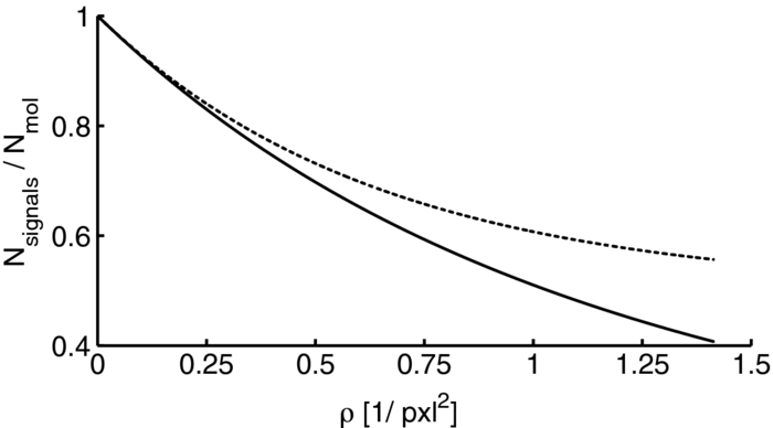

The monomer fraction α used in Sec. 4.2 is defined as p _cluster(1, w)/N _signals.

Appendix D: Limitations and Errors

The signal width w puts an upper limit on the density of signals: two molecules that approach each other by less than w cannot be resolved. The method presented here follows the molecules until bleaching and diffusion during that period leads to a broadening of the signal. For an immobile EYFP, we estimate a signal width of w = 160 nm. Including the broadening due to diffusion²⁵ with a diffusion constant of D = 0.8 μm²/s,¹⁵ the signal width becomes w = 178 nm. This small broadening does not hamper the applicability of the method in our experiments. In addition to long illumination times T, our method also requires that the bleaching time scale is much longer than the time scale of any blinking (see Appendix xA). In our experiments, blinking is obviously fast enough because we observe the exponential decay predicted for well-separated time scales. Different fluorophores might have blinking rates that are comparable to the bleaching rate. Such molecules cannot be used with our method.

We estimated the error for the measurement of the monomer fraction in Sec. 4.2 with the help of simulations. In particular, we assume that the mean number of emitted photons N is known and randomly generate N _signals signals with intensities drawn from the distribution [Eq. (8)]. The randomly drawn intensities are binned in equally sized bins, and the resulting distribution is normalized. This distribution is fit with [Eq. (8)] with α as the sole fit parameter. The whole procedure is repeated 100 times for each set of parameters, and the error is determined as the standard deviation Δα over the 100 values obtained for α. Figure 11 compares the influence of the experimental parameters on the relative error Δα/α determined by these simulations. Figure 11 A shows that Δα/α approximately scales like [TeX:] \documentclass[12pt]{minimal}\begin{document}$\propto 1 / \sqrt{N_{\rm{signals}}}$\end{document} $\propto 1 / \sqrt{N_{signals}}$ , which means that the accuracy can always be increased by measuring more signals. As expected, Δα/α increases with decreasing α. In Fig. 11b, we show that Δα/α scales approximately like ∝1/α. Δα/α is furthermore independent of the mean number of emitted photons N (data not shown).

Fig. 11

Accuracy of the measurement of the monomer fraction α determined from simulations. (a) Dependence of the relative error of α (solid circles) on the number of detected signals N _signals. A linear fit to the data in the log-log graph (solid line) has a slope of −0.49. N = 500, α = 0.5. (b) Dependence of the relative error of α (solid circles) on α. A linear fit to the data in the log-log graph (solid line) has a slope of −0.89. N = 500, N _signals = 5000.

The relative error we expect for the parameters of the experiment presented above (N = 837, N _signals ≈ 20000) ranges from 0.08 for α = 0.1 to 0.01 for α = 1. The errors we observe in experiments are much larger, (see inset of Fig. 5). The reason for that is twofold: First our simulations do not account for biological variability, which is probably considerable. Second, we combined data sets with different signal densities across intervals of width 0.02 μm⁻² (see inset of Fig. 5). Because the monomer fraction is decreasing quickly with signal density, heterogeneity within an interval contributes significantly to the reported error.

Acknowledgments

The authors thank Dr. S. Olthuis-Meunier for preparing the cell lines and Dr. J. Brzostowski for support on equipment for microscopy and data analysis. This work was supported by funds from the Stichting voor Fondamenteel Onderzoek der Materie of the Nederlands Organisatie voor Wetenschappelijk Onderzoek (NWO-FOM) within the program on Material Properties of Biological Assemblies (Grant No. FOM-L1707M).

References

1.

N. J. Leonard, R. Ghirlando, J. Askins, J. K. Bell, D. H. Margulies, D. R. Davies, and D. M. Segal, “The TLR3 signaling complex forms by cooperative receptor dimerization,” Proc. Natl. Acad. Sci. USA, 105 258 –263 (2008). https://doi.org/10.1073/pnas.0710779105 Google Scholar

2.

J. Schlessinger, “Ligand-induced, receptor-mediated dimerization and activation of EGF receptor,” Cell, 110 669 –672 (2002). https://doi.org/10.1016/S0092-8674(02)00966-2 Google Scholar

3.

P. H. M. Lommerse, B. Snaar-Jagalska, H. P. Spaink, and T. Schmidt, “Single-molecule diffusion measurements of H-Ras at the plasma membrane of live cells reveal microdomain localization upon activation,” J. Cell Sci., 118 1799 –1809 (2005). https://doi.org/10.1242/jcs.02300 Google Scholar

4.

J. Gandia, C. Lluis, S. Ferre, R. Franco, and F. Ciruela, “Light resonance energy transfer-based methods in the study of G protein-coupled receptor oligomerization,” BioEssays, 30 82 –89 (2008). https://doi.org/10.1002/bies.20682 Google Scholar

5.

T. Keppola, “Bimolecular fluorescence complementation (BiFC) analysis as a probe of protein interactions in living cells,” Annu. Rev. Biophys., 37 465 –487 (2008). https://doi.org/10.1146/annurev.biophys.37.032807.125842 Google Scholar

6.

M. A. Digman, R. Dalal, A. F. Horwitz, and E. Gratton, “Mapping the number of molecules and brightness in the laser scanning microscope,” Biophys. J., 94 2320 –2332 (2008). https://doi.org/10.1529/biophysj.107.114645 Google Scholar

7.

D. Kolin and P. Wiseman, “Advances in image correlation spectroscopy: measuring number densities, aggregation states, and dynamics of fluorescently labeled macromolecules in cells,” Cell Biochem. Biophys., 49 141 –164 (2007). https://doi.org/10.1007/s12013-007-9000-5 Google Scholar

8.

V. Vukojevic, M. Heidkamp, Y. Ming, R. Johansson, L. Terenius, and R. Rigler, “Quantitative single-molecule imaging by confocal laser scanning microscopy,” Proc. Natl. Acad. Sci. USA, 105 18176 –18181 (2008). https://doi.org/10.1073/pnas.0809250105 Google Scholar

9.

G. Malengo, A. Andolfo, N. Sidenius, E. Gratton, M. Zamai, and V. Caiolfa, “Fluorescence correlation spectroscopy and photon counting histogram on membrane proteins: functional dynamics of the glycosylphosphatidylinositol-anchored urokinase plasminogen activator receptor,” J. Biomed. Opt., 13 031215 (2008). https://doi.org/10.1117/1.2940570 Google Scholar

10.

T. Schmidt, G. Schütz, H. Gruber, and H. Schindler, “Local stoichiometries determined by counting individual molecules,” Anal. Chem., 68 4397 –4401 (1996). https://doi.org/10.1021/ac960710g Google Scholar

11.

T. McAnaney, W. Zeng, C. Doe, N. Bhanji, S. Wakelin, D. Pearson, P. Abbyad, X. Shi, S. Boxer, and C. Bagshaw, “Anomalous negative fluorescence anisotropy in yellow fluorescent protein (YFP 10C): quantitative analysis of FRET in YFP dimers,” Biochemistry, 44 5510 –5524 (2005). https://doi.org/10.1021/bi047581f Google Scholar

12.

M. H. Ulbrich and E. Y. Isacoff, “Subunit counting in membrane-bound proteins,” Nat. Methods, 4 319 –321 (2007). https://doi.org/10.1038/nmeth1024 Google Scholar

13.

L. Cognet, C. Tardin, M. L. M. Negrier, C. Breillat, F. Coussen, D. Choquet, and B. Lounis, “Robust single-molecule approach for counting autofluorescent proteins,” J. Biomed. Opt., 13 031216 (2008). https://doi.org/10.1117/1.2940600 Google Scholar

14.

L. Mandel, “Fluctuations of photon beams and their correlations,” Proc. Phys. Soc., 72 1037 –1048 (1958). https://doi.org/10.1088/0370-1328/72/6/312 Google Scholar

15.

P. H. M. Lommerse, G. A. Blab, L. Cognet, G. S. Harms, B. E. Snaar-Jagalska, H. P. Spaink, and T. Schmidt, “Single-molecule imaging of the H-Ras membrane-anchor reveals domains in the cytoplasmic leaflet of the cell membrane,” Biophys. J., 86 609 –616 (2004). https://doi.org/10.1016/S0006-3495(04)74139-9 Google Scholar

16.

M. Ormö, A. B. Cubitt, K. Kallio, L. A. Gross, R. Y. Tsien, and S. J. Remington, “Crystal structure of the Aequorea victoria green fluorescent protein,” Science, 273 1392 –1392 (1996). https://doi.org/10.1126/science.273.5280.1392 Google Scholar

17.

G. H. Patterson, D. W. Piston, and B. G. Barisas, “FÃrster distances between green fluorescent protein pairs,” Anal. Biochem., 284 438 –440 (2000). https://doi.org/10.1006/abio.2000.4708 Google Scholar

18.

T. Schmidt, G. J. Sch, W. Baumgartner, H. J. Gruber, and H. Schindler, “Imaging of single molecule diffusion,” Proc. Nat. Acad. Sci. USA, 93 2926 –2929 (1996). https://doi.org/10.1073/pnas.93.7.2926 Google Scholar

19.

Handbook of Single-Molecule Biophysics, Springer, New York (2009). Google Scholar

20.

G. S. Harms, L. Cognet, P. H. M. Lommerse, G. A. Blab, and T. Schmidt, “Autofluorescent proteins in single-molecule research: applications to live cell imaging microscopy,” Biophys. J., 80 2396 –2408 (2001). https://doi.org/10.1016/S0006-3495(01)76209-1 Google Scholar

21.

Y. Chen, J. Mueller, P. T. C. So, and E. Gratton, “Resolving heterogeneity on the single molecular level with the photon-counting histogram,” Biophys. J., 77 553 –567 (1999). https://doi.org/10.1016/S0006-3495(99)76912-2 Google Scholar

22.

K. Palo, U. Mets, V. Loorits, and P. Kask, “Calculation of photon-count number distributions via master equations,” Biophys. J., 90 2179 –2191 (2006). https://doi.org/10.1529/biophysj.105.066084 Google Scholar

23.

A. Papoulis, Probability, Random Variables and Stochastic Processes, McGRaw-Hill, New York (1991). Google Scholar

24.

S. Mutch, B. Fujimoto, C. Kuyper, J. Kuo, and S. Bajjalieh, “Deconvolving single-molecule intensity distributions for quantitative microscopy measurements,” Biophys. J., 92 2926 –2943 (2007). https://doi.org/10.1529/biophysj.106.101428 Google Scholar

25.

J. Schuster, F. Cichos, and C. von Borczyskowski, “Diffusion measurements by single-molecule spot-size analysis,” J. Phys. Chem. A, 106 5403 –5406 (2002). https://doi.org/10.1021/jp0144451 Google Scholar

Citation Download Citation

Tobias Meckel, Stefan Semrau, Thomas Schmidt, and Marcel J. M. Schaaf "Robust assessment of protein complex formation in vivo via single-molecule intensity distributions of autofluorescent proteins," Journal of Biomedical Optics 16(7), 076016 (1 July 2011). https://doi.org/10.1117/1.3600002

Published: 1 July 2011

Access the abstract

JOURNAL ARTICLE
14 PAGES

DOWNLOAD PAPER SAVE TO MY LIBRARY