2.1.

Model of Cylindrical Diffusing Fiber

Our diffuser model is based on a patent by E. L. Sinofsky,²⁵ whose construction is shown schematically in Fig. 1. It consists of four components: a fiber core, a diffusive medium, a dielectric reflector, and cladding. The fiber core is the 400 μm core of a 0.22 numerical aperture (NA) jacketed optical fiber. The diffusive medium consists of titanium dioxide (TiO₂) particles, with an average radius of 14.7 nm and an index of refraction of 2.488, embedded in a clear epoxy (Mastersil 151, Masterbond Inc., Hackensack, New Jersey) that has a density of 1 g/cm³ and a refractive index of 1.43.²⁵ The number density of TiO₂ particles providing a uniform axial fluence distribution is determined through simulation, as described in Sec. 3.1. The reflector is a dielectric stack, which is designed to provide maximum reflection with minimal heating. The cladding is a 0.25 mm layer of Teflon® FEP (DuPont, Wilmington, Delaware) with an index of 1.344 that surrounds the diffusive medium and dielectric reflector.

Fig. 1

Schematic of the cylindrical diffusing fiber, showing the four regions that are modeled. Photon packets are launched from the fiber core, with the diffusive medium being treated as having negligible absorption, and the cladding being treated as having negligible absorption and scattering. The dielectric reflector is treated as a perfect reflector.

Each of these four regions is modeled differently. The fiber core is treated as the launch point for photon packets, with packets being launched within the NA of the fiber. The face of the fiber core also serves as the detection point for fluorescence photon packets. Any fluorescence packet striking the fiber core within the NA of the fiber is recorded as being detected.

Since the diffusive medium consists only of TiO₂ spheres and a clear epoxy, it is treated as having negligible absorption. Photon propagation within the diffuser is therefore governed only by scattering. The bulk scattering coefficient (μ _s) within the diffusive medium depends on the concentration and size of the TiO₂ particles and is assumed to be uniform. This scattering coefficient must be optimized to achieve axially homogeneous irradiance along the diffuser length. In order to determine the optimal scattering coefficient for each diffuser length, μ _s was varied over a series of simulations and the homogeneity of the axial fluence profile was examined. The optimal value of μ _s was found by minimizing the deviation from an axially homogeneous fluence profile along the length of the diffuser.

The cladding layer consists of clear plastic and does not contain any scatterers. It is therefore treated as having negligible absorption and scattering. Therefore, this layer has the effect of inducing Fresnel reflection and transmission. The dielectric reflector is treated as a perfect reflector.

2.2.

GPU-Accelerated Monte Carlo Model

The propagation of photons is based upon the variance reduction MCML code by Wang ¹⁷ The movement, absorption, and scattering of photon packets are handled in the same way as in MCML. The code has been expanded to include the above diffuser model, a full 3D volume of optical properties, and fluorescence generation and detection.

Diffusers are specified by the three-dimensional coordinates, length, and radius of the diffusive region, and the outside radius of the cladding. Also specified are the NA of the fiber core, the scattering coefficient of the diffusive region, and the refractive indices of the diffusive region, and cladding. The total fluence to be delivered by the diffuser is specified in units of J/cm. An arbitrary number of these diffusers can be included in the simulation, with each diffuser able to launch photons and detect fluorescence. In the current version of the code, these diffusers are constrained to be parallel to the z-axis for simplicity. In clinical practice, diffusers are generally inserted in a parallel fashion,²⁶ so this limitation is not a major one.

For photon propagation, each photon packet is launched at a random location on the specified fiber core at a random angle that is within the NA of the fiber. In the diffusive region, the photon packet propagates by normal MC methods. This includes reflections off of the dielectric reflector and cladding. Since the scatterers present in the diffusive region are much smaller than a wavelength, the scattering can be treated as isotropic (g = 0), assuming random orientations of the scatterers and random polarization of the light. Upon transmission into the cladding, propagation continues without scattering or absorption. If the photon is transmitted into the surrounding tissue, propagation is continued as normal with the specified scattering and absorption in the tissue region.

Boundary interaction with the diffuser is done by monitoring the photon position with respect to the coordinates of the diffuser axis. If the current step size of the photon would take it either into or out of a diffuser, the coordinate system is temporarily converted to cylindrical coordinates. A random number is then compared to the Fresnel reflection coefficient for the boundary. If this random number is less than the reflection coefficient, the photon is reflected and propagation continues. Otherwise, the photon undergoes refraction and then continues propagation.

In order to represent the 3D tissue volume in which the diffuser is embedded, the simulation space is sub-divided into a matrix of cuboid voxels. Each of these voxels stores the absorbed weight at that location, scaled by the user-specified fluence and the size of the voxel, as well as an identifying region number. Each of these region numbers is tied to a set of optical properties that is specified by the user. These optical properties consist of the absorption coefficient (μ _a), the scattering coefficient (μ _s), the index of refraction, the scattering anisotropy (g), and the quantum yield of fluorescence if that region is fluorescent. These properties are specified at both the excitation and fluorescence emission wavelengths.

The 3D nature of the simulation also means that boundary reflections must be handled in three-dimensions. An excellent overview of this is given in Pfefer ²⁷ In our model, this is done by first determining all possible voxel boundaries that the photon packet will cross. The distance to each boundary is determined based on the current photon trajectory, and the region beyond that boundary is also recorded. The step size is then set to the shortest boundary distance that also leads into a different region. Reflection or transmission is determined based upon Fresnel coefficients, as described above, and photon propagation then continues. If the photon packet would not strike a boundary before executing its full step size, it is allowed to propagate its full step size.

During propagation of photon packets, fluorescence can be generated in the tissue. Whenever photon weight is absorbed, a fluorescence photon packet with a weight equal to the absorbed weight multiplied by the quantum yield of fluorescence is launched at that location. This fluorescence photon packet is immediately propagated by the above MC methods, but uses optical properties specified for the fluorescence emission wavelength. If a fluorescence photon packet strikes the fiber core inside the diffuser within the NA of the fiber, the photon is scored as detected. The position of its creation is recorded, as is the detected weight. This allows for the generation of a map of the origins of detected fluorescence photons, as well as what diffuser they were detected by in the case of an array of diffusers. This provides a description of regions that are sampled by spectroscopic measurements performed using the diffuser as a detector.

All of the above functions are performed on a GPU (GeForce GTX 570, NVIDIA Corporation, Santa Clara, California). It was programmed using NVIDIA's Compute Unified Device Architecture (CUDA) extensions to C. This allows for the code to run much faster than on a CPU. The GPU version of our model runs approximately 30 times faster than a CPU version of the same code. The parallel random number generator used in the code is based on that by Alerstam ²² This is required to ensure that photon packets being run simultaneously on separate threads use independent random numbers. The simulation parameters are stored in shared memory for faster access, while the absorption and detected fluorescence matrices are stored in the global device memory due to their large size. Atomic operations are required to update the absorption or detected fluorescence matrices in order to eliminate race conditions in memory access.

2.3.

Phantom Preparation

In order to validate the MC results, multilayered phantoms were created. These phantoms consisted of either two or three layers, as shown in Fig. 2. In both cases, the bottom layer was a solid layer comprised of agar. 500 mg of agar (SELECT Agar®, Invitrogen Corporation, Carlsbad, California) was added to 50 ml of de-ionized water and heated to 95 °C while stirring. Heat was then removed and the solution was stirred until the temperature fell to 80 °C. At this point, 5 mL of 10% Liposyn (Liposyn® II 10%, Abbott Laboratories, Abbott Park, Illinois), 14.6 μl of India ink (Higgins No. 4418, Chartpak Incorporated, Leeds, Massachusetts), and 36.6 μl of 1 mg/ml fluorescein (Sigma-Aldrich, St. Louis, Missouri) were added. Stirring continued until the solution reached 60 °C, at which point it was refrigerated at 5 °C overnight to solidify. The addition of this concentration of Liposyn provides a scattering coefficient of ∼90 cm⁻¹ at 488 nm.²⁸ Assuming a scattering anisotropy of 0.82, this produces a reduced scattering coefficient of 16.2 cm⁻¹. To ensure consistency, all phantoms were prepared from the same bottle of Liposyn. The addition of India ink brings the absorption coefficient to 2 cm⁻¹ at 488 nm. The amount of fluorescein added gives a fluorophore concentration of 2 μM. This will be referred to as the fluorescein layer.

Fig. 2

Experimental set-up for measurement of fluorescence in (a) two-layer and (b) three-layer phantoms. The diffuser was inserted such that each layer bordered on an equal length of the diffuser. Only one diffuser is shown for clarity, but experiments used two diffusers inserted in parallel with a separation of 1 cm. One diffuser was used for delivery of an axially homogeneous fluorescence excitation profile, while the other was used for detection of fluorescence.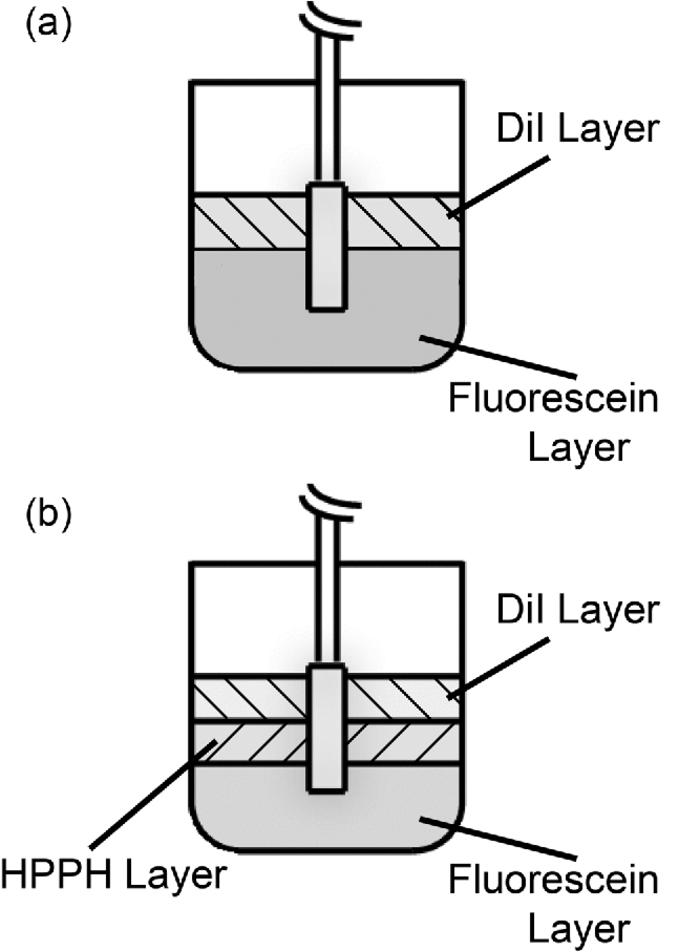

For the two layer phantom shown in Fig. 2a, the top layer was a liquid layer. This layer consisted of 10 ml of octanol (1-octanol, Sigma-Aldrich), 1 ml of 10% Liposyn, 2.8 μl of India ink, and 20.5 μl of 1 mg/ml 1,1^′-Dioctadecyl-3,3,3^′,3^′-tetramethylindocarbocyanine perchlorate (DiI) (Sigma-Aldrich). This was again designed to have a reduced scattering coefficient of 16.2 cm⁻¹, an absorption coefficient of 2 cm⁻¹, and a fluorophore concentration of 2 μM. This will be referred to as the DiI layer.

For the three layer phantom shown in Fig. 2b, the top layer was the DiI layer and the bottom layer was the fluorescein layer, both of which are described above. The middle layer consisted of 10 ml of 0.9% saline, 1 ml of 10% Liposyn, 3.06 μl of India ink, and 110.4 μl of 201.3 μM 2-[1-hexyloxyethyl]-2-devinyl pyropheophorbide-a (HPPH) dissolved in 1% Tween/phosphate buffered saline (PBS). HPPH is a second generation photosensitizer²⁹ that is also fluorescent. It was prepared for us by Ravindra Pandey at the Roswell Park Cancer Institute in Buffalo, New York, using the procedure described in Pandey ³⁰ This will be referred to as the HPPH layer.

Before use, each of the two liquid layers was stirred vigorously and poured on top of the fluorescein layer. Due to the immiscibility of octanol and saline solution, the DiI and HPPH layers remained distinct. HPPH is hydrophobic, but we dissolved it in Tween/PBS before diluting this solution in 0.9% saline. This keeps the HPPH confined to the saline solution, and we have seen no evidence of HPPH crossing into the DiI layer. Both liquid layers also remained distinct from the solid fluorescein layer.

2.4.

Experimental Validation of Simulated Fluorescence Detection by Diffusers

For fluorescence measurements, two diffusers were inserted parallel into the above phantoms, with a separation of 1 cm. For two layer experiments, two 1-cm diffusers (Pioneer Optics Company, Bloomfield, Connecticut) were inserted 0.5 cm into the fluorescein layer shown in Fig. 2a. The DiI layer was designed to have a depth of 0.5 cm when poured into a 150 ml flask, which meant that the proximal half of the diffuser was fully in the DiI layer and the distal half was fully in the fluorescein layer. Therefore, any detected DiI fluorescence is known to have been generated along the proximal half of the diffuser, and any detected fluorescein fluorescence is known to have been generated along the distal half of the diffuser.

For three layer experiments, two 1.5-cm diffusers (PhotoGlow Inc., South Yarmouth, Massachusetts) were inserted 0.5 cm into the fluorescein layer shown in Fig. 2b. Both the DiI and HPPH layers were designed to have a depth of 0.5 cm when poured into a 150 ml flask, which meant that the diffuser length was divided into three equal sections.

In both cases, excitation light at 488 nm was provided by an argon-ion laser (Innova 70, Coherent, Santa Clara, California), filtered by a band-pass filter (Z488Trans-pc-xr, Chroma Technology Corp, Bellows Falls, Vermont). Excitation light was delivered at 40 mW/cm for two-layer experiments and at 15 mW/cm for three-layer experiments. The optical power was lower for three-layer experiments due to larger coupling losses in the 1.5 cm diffusers. Optical power was measured using an integrating-sphere-based laser power measurement system (LPMS-060-SF-Si, Labsphere, North Sutton, New Hampshire). Excitation light was delivered through one of the diffusers in the experiment, and fluorescence was detected by the other. This was done to ensure homogeneous excitation along the diffuser length, and to minimize the detection of autofluorescence generated within the fiber. Light captured by the second diffuser was filtered through a long-pass filter (HQ500LP, Chroma) before being detected by a TE-cooled, 16 bit spectrometer (Compass X, B&W Tek, Newark, Delaware) using an integration time of 20 s.

For calibration purposes, fluorescence spectra were also collected from phantoms consisting of only one of the fluorophore layers. In order to do this, larger volumes of the layers described above were created while maintaining the concentrations of each component. This allowed the diffusers to be fully submerged in each layer.

2.5.

Data Correction and Spectral Fitting

All fluorescence spectra collected were corrected for background and system response. This was done by subtracting a dark measurement from the raw fluorescence measurement and dividing by a wavelength-dependent system response. Dark measurements were acquired by integrating dark signals for the durations described above. System responses were acquired by placing a single diffuser in the center of an integrating sphere (3P-LPM-060-SF, Labsphere) and shining a NIST-traceable lamp (Model No. LS-1-CAL, Ocean Optics, Dunedin, Florida) through one of the detection ports on the sphere. The measured spectrum was then background subtracted and divided by the known lamp spectrum to obtain the system response.

After fluorescence spectra were corrected, they were fit using a singular value decomposition (SVD) algorithm based on the work of Press ³¹ Basis spectra for each of the fluorophores were used in the fits. These basis spectra were acquired by measuring the fluorescence emission of each layer in a commercial fluorometer (Varian Eclipse, Palo Alto, California). In addition to the basis spectra, a series of 61 Fourier terms was also used in fitting to account for unknown possible contributions to the measured fluorescence. These Fourier terms were given a smaller weight in the fitting in order to favor the basis spectra. Fitting followed the SVD scheme found in MATLAB (Mathworks, Natick, Massachusetts).

After SVD fitting, the fit magnitudes for each fluorophore were further corrected for absorption and fluorescence yield effects. Each of the three fluorophores used has some absorption at 488 nm, and emits fluorescence beyond 500 nm. However, each fluorophore has different absorption at 488 nm and a different quantum yield of fluorescence. As mentioned previously, fluorescence spectra were acquired for each layer individually. These “pure” measurements were made using the same excitation wavelength and power as in the layered measurements, and with the same concentrations of scatterer, absorber, and fluorophore. So, any differences in absorption at 488 nm or fluorescence quantum yield were also present in the pure measurements. Therefore, any difference in magnitude between the pure and layered measurements was due to the detection capability of the diffuser at the height of the appropriate layer. To account for this, we divide the fit magnitude of the layered measurement by that of the pure measurement. This gives a relative measurement of the detected fluorescence that is weighted for absorption and fluorescence quantum yield.

3.1.

Determination of the Scattering Coefficient Within the Diffusive Region

As mentioned previously, the scattering coefficient within the diffuser determines the homogeneity of the axial fluence profile at the surface of the diffuser. If the value of μ _s is too large, most of the light launched from the fiber face will scatter out of the diffuser near the proximal end. If the value is too small, then the scattering out of the diffuser will be weak, which decreases the efficiency of the device. Figure 3 shows the simulated degradation in axial fluence profile for a 1 cm diffuser that is induced by use of an improper scattering coefficient. Figure 3a shows the homogeneous fluence profile along the surface of a 1 cm diffuser for the determined optimal value of μ _s = 0.2009 cm⁻¹ inside the diffuser. Figure 3b shows the effect of raising the value of μ _s to 10 cm⁻¹ within the diffuser, which results in too much light scattering out of the diffuser near the proximal end. The value of μ _s within the diffuser is therefore crucial to the generation of a homogeneous axial fluence profile.

Fig. 3

Simulated irradiance profiles along the surface of a 1 cm diffuser, with its proximal end at z = 1 cm, illustrating the effect of changing μ_s. Simulation parameters are identical in both cases except for the value of μ _s inside the diffusive region, which was (a) 0.2009 cm⁻¹ and (b) 10 cm⁻¹.

The optimal μ _s for homogeneous axial fluence changes with diffuser length. The optimal μ _s values computed using our MC model for diffuser lengths between 1 and 5 cm are shown in Table 1. As can be seen, the required μ _s for homogeneous fluence decreases with increasing diffuser length. This corresponds to a reduced concentration of scatterers through μ _s = σN, where σ is the scattering cross-section and N is the number density of scatterers.³² The scattering cross-section can be calculated using

Fig. 9

Comparison between simulated and experimental fluorescence detection using (a) 1 cm and (b) 1.5 cm diffusers. Heights of experimental bars (□) indicate the mean value of (a) n = 6 and (b) n = 4 experiments, with error bars representing standard deviation. Values used were corrected for background, system response, fluorescence quantum yield, and absorption at 488 nm. Heights of simulated bars (■) indicate the mean value of 3 simulations, with error bars representing the standard deviation. The value of μ _a was set to 2 cm⁻¹ for both simulation and experiment.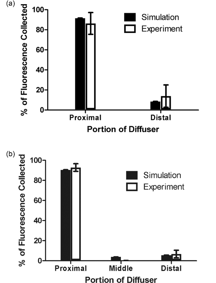

Table 1

Optimal scattering coefficient (μ s) for homogeneous irradiance for multiple diffuser lengths, and the corresponding calculated number density of scatterers (N). N is given in units of cm−3 and ppm by weight. Number densities in ppm by weight used in commercial diffusers manufactured by Pioneer Optics Company are shown for comparison.

3.2.

Fluence Distributions Generated by Monte Carlo Model of Diffuser

A typical fluence map generated by a 1 cm diffuser is shown in Fig. 4. The air-tissue boundary is located at z = 0, and the proximal end of the diffuser is at z = 0.5 cm. For this particular simulation, the tissue sample is homogeneous and semi-infinite with μ _a = 2 cm⁻¹, μ _s = 100 cm⁻¹, g = 0.9, and n = 1.395 (Ref. 34).

Fig. 4

3D rendering of the fluence distribution around a 1 cm cylindrical diffusing fiber with its proximal end at z = 0.5 cm and an air-tissue boundary at z = 0. Tissue optical properties were set to μ _a = 2 cm⁻¹, μ _s = 100 cm⁻¹, and g = 0.9. Voxel size was 0.02×0.02×0.02 cm.

In order to compare to a model based on a finite linear array of point sources, the radial degradation of fluence from the diffuser was examined for both models. In these simulations, we assumed a refractive index of 1.43 for the linear array to match that of the epoxy in the diffuser. Cuts through the fluence distribution were made radially from the axial mid-point of the diffuser for both models. The results of this are shown in Fig. 5. As can be seen, the fluence cuts are virtually identical for the two models. Similar results were obtained for cuts at other axial positions on the diffuser, and at other angles (data not shown). This indicates that a model based on a linear array of point sources is sufficient for determination of fluence distribution.

Fig. 5

Comparison between linear array of point sources model and our MC model in terms of radial degradation of fluence for μ _a = 2 cm⁻¹, showing substantial overlap between the two methods. Shown is a cut through the fluence at the axial center of a 1 cm diffuser. Simulation parameters were identical, except for the source model. The arrow indicates the position of the outer radius of the diffuser.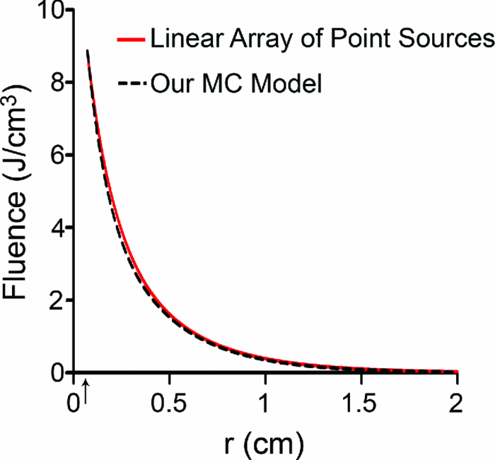

3.3.

Modeling of Fluorescence Generation and Detection

As mentioned previously, fluorescence photon packets are generated at the location of each absorption event within the tissue medium surrounding a diffuser. Generated fluorescence photon packet weights consist of the absorbed weight, scaled by the quantum yield of fluorescence. Therefore, the distribution of generated fluorescence is a scaled version of the absorption distribution. This is shown in Fig. 6a for a 1 cm diffuser. As expected, this generated fluorescence is homogeneous along the length of the diffuser. Figure 6b shows the origins and weights of generated fluorescence photons that cross into the diffuser. This is simply a scaled version of the generated fluorescence, and is again homogeneous along the length of the diffuser. The distribution of the origins of detected fluorescence photon packets is shown in Fig. 6c. Each pixel magnitude is the sum of the detected weight of fluorescence photon packets generated at that location that migrated through the diffuser, reached the fiber core, and were scored as detected. This distribution is highly heterogeneous, with a majority of the detected fluorescence being generated near the proximal end of the diffuser.

Fig. 6

(a) Fluorescence generated in tissue by a 1-cm diffuser with its proximal end at z = 2 cm and an outer radius of 0.05 cm. (b) Origins of fluorescence photons that crossed into the diffuser after being generated in the surrounding tissue. (c) Origins of fluorescence photons that were detected by the diffuser. μ _a was set to 2 cm⁻¹ in tissue. Planar cuts are shown through the simulated volume at the center of the diffuser. Only the right half of this plane is shown for clarity. The left half is identical.

Axial profiles of the simulated detected fluorescence are shown in Fig. 7. These profiles were created by summing the detected fluorescence at each z position within the simulated tissue volume. Optical properties of the tissue sample were set to μ _s = 90 cm⁻¹, g = 0.82, and n = 1.395, with either μ _a = 2 cm⁻¹ to match experimental conditions or μ _a = 0.2 cm⁻¹ to represent a typical value in tissue.³⁵ As can be seen, the majority of detected fluorescence comes from the proximal portion of the diffuser, with a slightly increased contribution from the distal portion of the diffuser relative to the center. Detected fluorescence, detailed by the diffuser segment, is shown in Table 2. In all cases, the majority of detected fluorescence comes from the proximal third of the diffuser, with contributions ranging from 86 to 92% for μ _a = 2 cm⁻¹ and from 70 to 88% for μ _a = 0.2 cm⁻¹. In all but the 1 cm case for both values of μ _a and the 1.5 cm case for μ _a = 2 cm⁻¹, the distal third of the diffuser is responsible for the next largest contribution to detected fluorescence, with the center segment having the smallest contribution. Relative fluorescence collection by the distal third ranges from 5.38 to 6.66% for μ _a = 2 cm⁻¹ and 9.11 to 11.98% for μ _a = 0.2 cm⁻¹, with the center section collecting 1.63 to 6.11% for μ _a = 2 cm⁻¹ and 2.03 to 18.15% for μ _a = 0.2 cm⁻¹.

Fig. 7

Simulated detected fluorescence by axial position along (a) 1 to 2 cm diffusers with μ _a = 2 cm⁻¹, (b) 3 to 5 cm diffusers with μ _a = 2 cm⁻¹, (c) 1 to 2 cm diffusers with μ _a = 0.2 cm⁻¹, and (d) 3 to 5 cm diffusers with μ _a = 0.2 cm⁻¹. All simulations used μ _s = 90 cm⁻¹ and g = 0.82, and placed the diffuser's proximal end at z = 0.5 cm. The arrows indicate the location of the proximal end of the diffusers.

Table 2

Percentage of generated fluorescence that is collected by various segments of different diffuser lengths, as determined by our MC model. Thirds correspond to the three-layer experiment, and halves correspond to the two-layer experiment. Uncertainties given are the standard deviation of three successive runs of the simulation.

Simulations were run with 1,000,000 photon packets on a 100×100×100 grid of voxels. Due to the statistical nature of MC modeling, simulations were repeated three times in order to evaluate reproducibility. The variation in detected fluorescence varies by at most 4% between runs, with most values varying by less than 1%. The run-times were approximately 1 min for simulations of fluence distribution and approximately 30 min for simulations of fluorescence detection.

3.4.

Experimental Validation of Fluorescence Detection

Experiments were performed in two- and three-layer phantoms with 1 and 1.5 cm diffusers, respectively. Typical SVD fits to corrected fluorescence spectra are shown in Fig. 8. The two-layer fit in Fig. 8a shows contributions from DiI and fluorescein, while the three-layer fit in Fig. 8b shows contributions from DiI, fluorescein, and HPPH. In both cases, the magnitude of the Fourier terms is relatively small, indicating a good fit to the data.

Fig. 8

Results of SVD fitting to representative fluorescence spectra collected from (a) two-layer and (b) three-layer phantoms, with spectra corrected for background and system response. Fit magnitudes shown are not corrected for the effects of fluorescence quantum yield and absorption at 488 nm.

Fit coefficients for the fluorophores were further corrected for absorption and fluorescence quantum yield as described above. The corrected values were then used to determine the relative contributions of each segment of the diffuser to the overall detected fluorescence. The results of this are shown in Fig. 9, with the simulated values shown for comparison. For both two- and three-layer experiments, there is agreement between the simulation and experiment to better than 6%. The results shown are for a set of 6 two-layer experiments, and a set of 4 three-layer experiments. Error bars are standard deviations. Error bars for simulated data are the standard deviations from three successive runs of the simulation.