
|
|
1.IntroductionAn optical inhomogeneity in turbid media (e.g., soft tissue) may imply the existence of a hemorrhage, tumor, or high saturation of oxygenation in a case where absorption and/or scattering characteristics of tissue changes with respect to the concentration of the natural chromophore. For detection and localization of such optical inhomogeneities, illumination with nonionizing electromagnetic (EM) radiation in near-infrared (NIR) or visible region has been utilized. Specifically EM radiation (600 to 1000 nm) is weakly absorbed inside the biological tissue by experiencing many scattering events per unit length, diminishing the availability of detecting ballistic photons.1, 2 NIR radiation is used in diffuse optical imaging (DOI) or tomography (DOT), which is a medical imaging modality to obtain optical parametric maps of living tissue.3, 4, 5, 6 The main idea in DOT is the reconstruction of the probed volume by solving a forward model of photon propagation iteratively3, 4, 5 and to map spatially resolved spectroscopic chromophore concentrations.7, 8, 9, 10 Even though DOT has great advantages, namely use of safe wavelengths, repetitive use, portability, and low cost, it suffers from low spatial resolution with respect to other imaging modalities such as x ray tomography, MRI, and ultrasound imaging.11, 12, 13 Recently, it has been proposed that the location of a defect inside a turbid medium obtained by a direct localization method could be used as a priori spatial information for recursive algorithms in DOT.14, 15 Direct localization schemes generally depend on transillumination measurements, which can be used for slab, finite-size, 14, 16, 17, 18, 19, 20, 21 or circular geometries.15 In contrast, for diffuse reflectance measurements, only a few schemes were proposed to improve the accuracy in localization.22, 23, 24 Time domain (TD)23, 24 and frequency domain (FD) measurements22 which are complicated with respect to cw measurements11 have attempted to address this issue but no method exists for the fastest and inexpensive method that uses the cw approach. Knowledge on the depth of an absorber could be incorporated in the process of selecting optimal regularization parameters in both cw and frequency-domain DOI.25, 26 Adapting the modulation frequency in accordance to the known depth coordinates allows increased specificity and sensitivity in DOI27 and increase in image resolution.28, 29, 30, 31, 32 Underdeterminacy of the DOI could also be reduced by introduction of an adaptive grid mesh in the reconstructed volume of interest.15, 33 However, co-registration of images from different modalities has subtleness,33, 34 and different imaging modalities assess the size of the defects (lesions) differently,35 probably due to the inherently different contrast mechanisms in operation.33, 36 The goal of this paper is to recommend a strategy to estimate the depth of an absorber inside a turbid medium. We address the challenge via a single wavelength spatially resolved continuous wave (SRCW) diffuse reflectance for semi-infinite geometry and show that under various probe geometries and optical parameters, it is possible to localize the depth of the absorber to within 0.1-mm precision. The accuracy of the method is analyzed for different combinations of optical properties of the absorber and the medium, as well as for different spatial placement of the cw source and detectors on the surface of the medium. 2.TheoryAn optical defect (absorber) residing in a turbid medium introduces a perturbation to NIR light propagation that is represented as a decrease in measured response. Physically the perturbation is a function of the distance between the defect and the detector when the source and the detector positions are fixed. For a configuration of a single source and multiple detectors in a row (Fig. 1), the perturbation will be less at the farther detectors as long as the defect resides between the source and the closest detector. We propose a method to extract the depth information from the differential effect of perturbation on multiple detectors in a row. Fig. 1The method consists of a cw source (S) and the measurement of diffuse reflectance at two distances. The source, proximal, and the distal detectors are located on a row (y = 0). The defect resides between the source and the proximal detector. SPD: source-proximal detector distance; ID: interdetector distance; SCX: x component of source-center of the defect distance. The origin of Cartesian coordinate system is the location of the source and +x, +y, and +z are as shown.  In this study, a solution of time-independent diffusion equation of photon propagation in turbid media is used for simulations.37 This solution is derived for the case where the semi-infinite medium is illuminated by a cw source. The response of a medium containing a spherical inhomogeneity is referred to as the perturbed response [literally total photon-flux-density (J T) in units of detected photons per unit area per unit time at the measurement site]. J T is the summation of two components J 0 and J 1, the response of the unperturbed background medium, and the perturbation introduced by a spherical defect respectively.37 Eq. 1[TeX:] \documentclass[12pt]{minimal}\begin{document}\begin{equation} J_0 = \delta |\vec E_0 (\vec r)|, \end{equation}\end{document}Eq. 2[TeX:] \documentclass[12pt]{minimal}\begin{document}\begin{equation} \vec E_0 \left({\vec r} \right) = \frac{{z_0 S_0 }}{{2\pi \delta }}\left({\frac{{3\kappa z\vec r}}{{r^4 }} + \frac{{3z\vec r}}{{r^5 }} {-} \frac{{\kappa \hat z}}{{r^2 }} {-} \frac{{\hat z}}{{r^3 }} {+} \frac{{\kappa ^2 z\vec r}}{{r^3 }}} \right){\rm exp}\left({ - \kappa r} \right){\rm}, \end{equation}\end{document}The perturbation by the spherical defect at the detector site (J 1) is: Eq. 3[TeX:] \documentclass[12pt]{minimal}\begin{document}\begin{eqnarray} \begin{array}{l} \hspace*{-3pt}J_1 = 2\delta q\displaystyle\frac{{\left({\kappa \left| {\vec r_c - \vec r_d } \right| + 1} \right)}}{{\left| {\vec r_c - \vec r_d } \right|^3 }}\exp \left({ - \kappa \left| {\vec r_c - \vec r_d } \right|} \right)\phi _0 \left({\vec r_c } \right) \\[8pt] \hspace*{15pt} - 2\delta p\left\{ {\displaystyle\frac{{[ {\left({\vec r_c - \vec r_d } \right)\,\vec E_0 \left({\vec r} \right)} ]\left({\kappa \left| {\vec r_c - \vec r_d } \right| + 3} \right)z_c }}{{\left| {\vec r_c - \vec r_d } \right|^5 }} - \displaystyle\frac{{E_0 \left({\vec r_c } \right)}}{{\left| {\vec r_c {-} \vec r_d } \right|^3 }}} \right\}\\ \quad\,\,\,\,\,\times\,\exp \left({ - \kappa \left| {\vec r_c {-} \vec r_d } \right|} \right), \end{array}\hspace*{-10pt}\nonumber\\ \end{eqnarray}\end{document}Some of the properties of the multiplicands q and p are to be stressed. When [TeX:] $\tilde \mu _a$ = μa, q is zero. On the other hand, such a relation does not exist for p when [TeX:] $\mu^ \prime _s$ = [TeX:] $\tilde \mu^ \prime _s$ . It has been reported that an absorber embedded in a semi-infinite medium modifies cw diffuse reflectance such that a shadow on the measurement surface appears.38 Methods depending on this idea have been shown to detect the projection of a single defect or two defects onto the measurement surface for the semi-infinite geometry; at the expense of multiple measurements with spatially resolved sampling. 3.Methods3.1.General Approach3.1.1.Generation of ratio-versus-depth curveAs it was reported by Feng, if q is nonzero (for [TeX:] $\mu _a \ne \tilde \mu _a$ ) in Eq. 3, the term with multiplicand q is dominant in practice.37 When the Eq. 3 is truncated as: Eq. 4[TeX:] \documentclass[12pt]{minimal}\begin{document}\begin{equation} J_1 \approx 2\delta q\frac{{\left({\kappa \left| {\vec r_c - \vec r_d } \right| + 1} \right)z_c }}{{\left| {\vec r_c - \vec r_d } \right|}}\exp \left({ - \kappa \left| {\vec r_c - \vec r_d } \right|} \right)\phi _0 \left({\vec r_c } \right) \end{equation}\end{document}Eq. 5[TeX:] \documentclass[12pt]{minimal}\begin{document}\begin{equation} \frac{{J_1^P }}{{J_1^D }} = \frac{{2\delta q\frac{{\left({\kappa \left| {\vec r_c - \vec r_d^P } \right| + 1} \right)z_c }}{{\left| {\vec r_c - \vec r_d^P } \right|^3 }}\exp ({ - \kappa | {\vec r_c - \vec r_d^P } |})\phi _0 \left({\vec r_c } \right)}}{{2\delta q\frac{{\left({\kappa \left| {\vec r_c - \vec r_d^D } \right| + 1} \right)z_c }}{{\left| {\vec r_c - \vec r_d^D } \right|^3 }}\exp ({ - \kappa | {\vec r_c - \vec r_d^D } |})\phi \left({\vec r_c } \right)}}, \end{equation}\end{document}Eq. 6[TeX:] \documentclass[12pt]{minimal}\begin{document}\begin{equation} \frac{{J_1^P }}{{J_1^D }} = \frac{{\frac{{\left({\kappa \left| {\vec r_c - \vec r_d^P } \right| + 1} \right)}}{{\left| {\vec r_c - \vec r_d^P } \right|^3 }}\exp ({ - \kappa | {\vec r_c - \vec r_d^P } |})}}{{\frac{{\left({\kappa \left| {\vec r_c - \vec r_d^D } \right| + 1} \right)}}{{\left| {\vec r_c - \vec r_d^D } \right|^3 }}\exp ({ - \kappa | {\vec r_c - \vec r_d^D } |})}}. \end{equation}\end{document}Since the placement of detectors can be arranged, the components of detector vectors ( [TeX:] $\vec r_d^P$ and [TeX:] $\vec r_d^D$ ) are fully known. Operands of κ (μa and [TeX:] $\mu^ \prime _s$ ) can be assessed by optical methods in vivo. 39, 40, 41, 42, 43, 44, 45 Please note that z c in Eq. 5 cancels out in Eq. 6. The depth information of the center of the defect remains as a Cartesian component of [TeX:] $\vec r_c$ with respect to origin – x c, y c, and z c. Assuming that the planar coordinates (x c and y c) of the defect relative to the source are known,46 depth (z c) remains the only unknown independent variable on the right-hand side of Eq. 6 implicit in [TeX:] $\vec r_c$ . A curve generated by Eq. 6 for a range of z c (typically from 5.0 to 40.0 mm) is referred as the ratio-versus-depth curve throughout the text. The generation of ratio-versus-depth curve does not include the knowledge of absorption coefficient of the defect ( [TeX:] $\tilde \mu _a$ ) and radius of the defect (a). In this study, for all cases, the location of proximal detector with respect to source is arranged such that the defect always resides between the source and the proximal detector. Both the source and detectors are taken as extended source and detectors of 1 mm2 core-area to have a realistic calculation. 3.1.2.Depth estimationOptically turbid medium is considered to contain an absorbing spherical defect whose scattering coefficient is the same as the medium (Fig. 1). The ratio of perturbed responses of the medium measured at the proximal and distal detectors is: Eq. 7[TeX:] \documentclass[12pt]{minimal}\begin{document}\begin{equation} R = \frac{{\left({J_0^P + J_1^P } \right)}}{{\left({J_0^D + J_1^D } \right)}}. \end{equation}\end{document}Eq. 8[TeX:] \documentclass[12pt]{minimal}\begin{document}\begin{equation} R = \frac{{\left({J_0^P + J_1^P } \right) - J_0^P }}{{\left({J_0^D + J_1^D } \right) - J_0^D }} = \frac{{J_1^P }}{{J_1^D }}. \end{equation}\end{document}Fig. 2Schematic view for the depth estimation and error calculation. The solid line corresponds to ratio-versus-depth curve, which is generated by Eq. 6. Stars on the graph show exact ratio values (rarefied for clearance) obtained by Eq. 3 with the same parameters and the set of depth values. For the exact depth A first, y 1 is calculated and y 1 is projected into horizontal axis to B via the ratio-versus-depth curve. Hence, the error at depth A is the absolute value of A-B divided by the diameter of the defect. For the depth D, the error is the absolute value of C-D divided by the diameter of the defect. 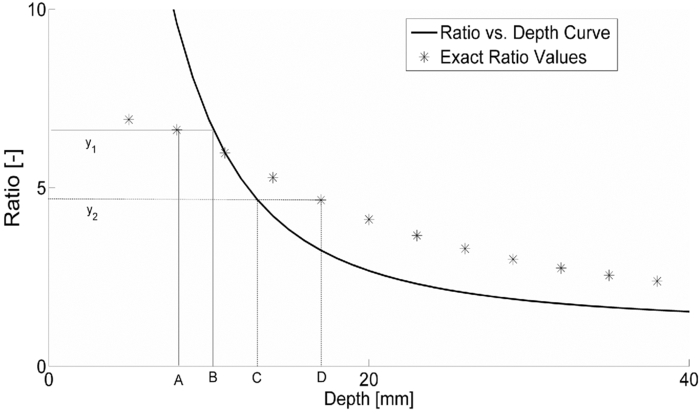 Knowledge on the unperturbed response is required for the application of the proposed method. The method is further extended (described in Sec. 3.4) for the cases where the unperturbed response might be erroneously calculated. 3.2.Analysis of the Proposed MethodThe distance from the source to the planar location of the defect (SCx), source-proximal-detector distance (SPD), and interdetector distance (ID) can be adjusted according to physical conditions (Fig. 1). Absorption coefficient and radius of the defect (a) do not take part in the generation of ratio-versus-depth curves [Eq. 6], but still can influence the results since they are present in Eq. 3. Therefore, the analysis of the method comprises two approaches. First, the effect of placement of source and detectors on ratio-versus-depth curves, second, the precision of the depth estimation under different probe placement for different defect size and defect/background medium absorption coefficient are analyzed. The geometry used to derive ratio-versus-depth curves is shown in Fig. 1. Even if the defect is a pure absorber ( [TeX:] $\mu^ \prime _s$ = [TeX:] $\tilde \mu^ \prime _s$ ), the frequency of scattering events inside the defect are increased compared to the background. This could be attributed to light-tissue interaction results from simultaneous scattering and absorption.1 The precision of the method is tested quantitatively by calculating error introduced by the approximation [setting p = 0 in Eq. 3]. The error is defined as follows: for a particular depth of the center of defect (e.g., point A in Fig. 2), the exact ratio (y 1) is calculated by the exact formula [Eq. 3] and plotted as the point (A, y 1) in Fig. 2. The ratio-versus-depth curve [by Eq. 6] obtained by the same geometry and optical properties is plotted on the same graph. The exact ratio (y 1) is projected onto the depth axis to obtain assessed depth via the ratio-versus-depth curve (point B in Fig. 2). Hence, the error at depth A is obtained by dividing the absolute value of the difference between A and B with the diameter of the defect. The divisor is chosen as the diameter of the defect to compare cases with different defect sizes and to avoid depth dependence on the error. For the quantitative analysis of the method, the errors are calculated for different sets of ID, SCx, z c , background medium, and defect optical parameters (Fig. 3). Additionally, we studied the error introduced due to possible mistakes in lateral coordinates (Fig. 4). Errors are shown with filled-contour matrices as a function of z c and SCx (Figs. 3, 4). Fig. 3Error maps for four different situations. In general, placing the source directly above or close to the defect minimizes the error introduced by the scattering effect (error < 0.05). On the other hand, the ratio values corresponding to the superficial regions of the medium are more likely to contain a scattering effect (a)–(d). (b) Change in ID distorts the overlap of banana shaped SSPs of the proximal and the distal detector. Increasing ID (from 2.5 to 10.0 mm) does not change the error distribution when SCX < 25.0 mm. (c) Defects with bigger size (5.0 mm instead of 2.0 mm) may introduce higher errors when the proximal detector is close to the defect. (d) Increase in μ a (from 0.005 to 0.050 mm−1) does not change the error distribution but decreases error values. S: Source PD: Proximal Detector.  Fig. 4Error maps for off-center placement. Simulations are generated with the same parameters as in Table 1. Errors in depth estimation are below 0.10 for defects deeper than 10 mm and higher than 20 mm in the turbid media. The profile of error distribution is similar for different interdetector distances (b), defects with different sizes (c), or media with different μ a (d). S: Source.  Fig. 9Averages and standard errors of measurement of perturbed response as a function of the depth of the center of the defect. (a) Solid and dottted lines correspond to measurements of detectors at 20.0 and 30.0 mm distance with respect to source. Standard errors of both curves are very small with respect to average values. Experimental values are averages of seven measurements whose standard errors are shown. (b) Experimentally obtained ratio values are shown by squares and solid curve is the ratio-versus-depth curve. (c) Schematic views of measurement cross section. The light gray portion depicts the aquarium filled with intralipid solution. The dark gray square is the defect (cube). Black dot inside the dark gray square shows the center-of-mass of the cube and white dot is the assessed depth. Deviations from left to right: 16.0−0.93 mm; 24.0+0.48 mm; 32.0+2.34 mm; 40.0−2.24 mm.  Table 1Parameters used for error calculation in Figs. 3a, 3b, 3c, 3d, 4a, 4b, 4c, 4d. Parameters used for simulations in Fig. 5. 3.3.Analysis of Probable Errors in Experimental ConditionsThe necessity to calculate the response of the background (J 0) might be a limiting factor in the applicability of our method for cases where the relatively accurate knowledge on the background optical properties is not available either experimentally or from the literature. A set of optical parameters (predicted from the literature) can be used in iterative algorithms. One approach to use for iterations might be to measure the response of the probed medium with an array of detectors for a configuration in which the defect does not reside between the source and detectors. The erroneous prediction or estimation of the medium optical parameters is studied and an extension of the method is suggested for improved depth assessment. To analyze this case, the measured response is simulated by feeding a set of optical parameters (actual μa and [TeX:] $\mu^ \prime _s$ ) to Eq. 3. Then, the unperturbed response of the medium (J 0) is calculated for a range of μa and [TeX:] $\mu^ \prime _s$ selected around the “actual” values and a matrix of calculated ratio values is obtained. The physical constraints require two conditions to be satisfied. First, for each detector (both proximal and distal) the measured response must be less than the corresponding calculated J 0. Second, the effect of perturbation must be greater at the proximal detector compared to the distal one (ratio values greater than one). The upper limit of the calculated J 0 was set not to be higher than three folds of the measured response physically.37 The first step is to exclude the set of parameters with a nonphysical outcome from the matrix. The candidate set of optical parameters is then used to estimate the depth of the defect from the corresponding ratio-versus-depth curves for spatially resolved measurements. The next step is to compare the depth values within matrices obtained from different measurements. The depth estimation with smallest standard deviation for the assessed depth values is taken to correspond to the one obtained with the optical values closest to the actual ones (Fig. 5). Fig. 5Windowing of scattering and absorption parameters of the unperturbed background response. (a) Schematic representation of the source-detector array configuration. M1–M4 the individual measurements used for depth estimation. (b) The x and y axis show the range of the absorption coefficient and reduced scattering coefficient, respectively. Only the minimum–maximum and actual values are represented near axes. In this case a matrix of 42 × 41 is shown. The black and white dots are nonphysical and physical results respectively. The optical parameter set selected to simulate the measured response is represented by a white square. Optical parameter set estimated from the depth values with minimum standard deviation is recognized with a cross. The simulation parameters are stated in Table 1. Interdetector distance is 2.5 mm for all measurements (M1–M4).  3.4.Experimental Material and Experimental ProcedureAn aquarium with darkened sides with dimensions 100.0 × 100.0 × 100.0 mm is filled with 1% intralipid. The aquarium is made of PVC and the top of the aquarium is drilled to hold the 1.1 mm core diameter (whose area is taken as 1.0 mm2) fibers as sources and detectors. A 1-kHz frequency signal is used to operate a 3 mW, 785 nm diode laser (RLD78MA-E Thorlabs). A lock-in amplifier is used to lock the signal to the chosen frequency and eliminate the noise (SRS SR510 Stanford Research). The optical properties of the intralipid solution used in the experiment are μa = 0.002 mm−1 and [TeX:] $\mu^ \prime _s$ = 0.827 mm−1 by measurement. A 1.0 cm3 dark gray cubical rubber is placed at the symmetrical center between source and detector fibers. The source-proximal detector distance is 20.0 mm and the interdetector distance is 10.0 mm to avoid the effect of field-of-view of detectors on measurements.47, 48, 49 The source-center of the defect distance is 10.0 mm. Diffuse reflectance values are obtained via descending the rubber by a step size of 1 mm starting at 15 to 40 mm (with respect to the center of the rubber from the sample-ambient layer boundary). The depth range chosen enabled to make measurements of enough intensity. The J 0 is obtained by measuring spatially-resolved reflectance after the cube is removed from the aquarium. 4.Results4.1.Simulation ResultsThe diffusely reflected photons injected into a semi-infinite turbid medium by a cw source, traverses the medium in the shape of banana to reach a detector.50 The banana-shaped spatial sensitivity (SSP) profile moves toward the medium-air interface with a sharper peak and narrower distribution51 when the absorption coefficient of the medium increases. Since the volume of the defect is small with respect to volume probed, the banana-shaped SSP will be used qualitatively in this study. The optical parameters used in this study are selected to resemble typical in vivo parameters for biological tissue cited in literature2 (Tables 1, 2). Absorption contrast between the defect and the background medium is fourfold in accordance with previous studies.52 Table 2Parameters used for curve generation in Figs. 6, 7, 8.
The relative placement of detectors and the source with respect to planar position of the defect is an important parameter since different combinations yield different ratio-versus-depth curves (Figs. 6, 7, 8). The effects of different values for source-center of the defect distance (SCx), ID, and SPD are studied in this work (Table 2). Fig. 6Ratio-versus-depth curve generated for different source-center of the defect distance (SCx). Five distances are used: 0.0, 5.0, 10.0, 15.0, and 20.0 mm. (a) Top views of simulated geometries are depicted. S: Source, PD: proximal detector, DD: distal detector. Irregular gray shape symbolizes the defect. From top to bottom, SCx = 20.0, 15.0, 10.0, 5.0, and 0.0 mm. (b) The effect of SCx on ratio-versus-depth curves are displayed, where dashed curve/circle (SCx = 0.0 mm), dashed-dotted/diamond (SCx = 5.0 mm), dotted/cross (SCx = 10.0 mm), thin-solid/triangle-ups (SCx = 15.0 mm) and thick-solid/triangle-downs (SCx = 20.0 mm). SPD = 20.0 mm; ID = 2.5 mm.  Fig. 7The effect of SPD on ratio-versus-depth curve. (a) Top views of simulated geometries are displayed. Irregular gray shape symbolizes, defect, S is the source, PD and DD are proximal and distal detectors, respectively. For the two geometries in the bottom, labels are not drawn. From top to bottom: SPD = 10.0, 20.0, and 30.0 mm. ID = 2.5 mm and the source is directly placed above the defect. (b) ratio-versus-depth curves and exact ratio values are displayed. Ratio-versus-depth curve/exact ratio values are displayed in pairs: Dashed-doted curve/cross (SPD = 30.0 mm), dashed curve/triangle-ups (SPD = 20.0 mm), solid curve/triangle-downs (SPD = 10.0 mm). SCx = 0.0 mm; ID = 2.5 mm. When the PD is placed relatively farther, the perturbations in detectors become close to each to other. 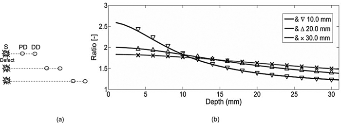 Fig. 8Ratio-versus-depth curves for different ID. (a) Four different cases depicted in the top views of geometries, from top to bottom, ID = 10.0, 7.5, 5.0, and 2.5 mm, respectively. S shows the source, PD is the proximal, and DD is distal detector. Irregular gray shape symbolizes the defect in all cases. (b) The ratio-versus-Depth curves and exact ratio values are displayed pair wise: dashed-dotted curve/circle (ID = 2.5 mm), dotted curve/triangle-ups (ID = 5.0 mm), dashed curve/cross (ID = 7.5 mm), solid curve/triangle-down (ID = 10.0 mm). SCX = 0.0 mm; SPD = 20.0 mm. For the SPD of 20.0 mm, ratio-versus-depth curves match better with exact values. As expected, when the distance between PD and DD is longer, the perturbation measured at PD becomes more than that at DD. 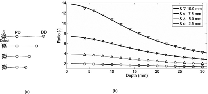 Ratio-versus-depth curves are generated [Eq. 6] for a range of defect depth from 1 to 30 mm with a step size of 1 mm (Figs. 6, 7, 8). To visualize the effect of the neglected term, ratio values obtained by the exact relation given in Eq. 3 are displayed in the same figures (Figs. 6, 7, 8). Used optical and geometrical parameters are displayed in Table 2. For each set of parameter, depths of the center of the defect are taken from 4 to 30 mm with a step size of 2 mm (14 values in Figs. 6, 7, 8). In a fixed constellation of source relative to the detectors (constant SPD and ID) it is possible to construct ratio-versus-depth curves with different characteristics via changing the placement of the source relative to the planar position of the defect (Fig. 6). As SCx approaches SPD, the perturbation at the proximal detector increases resulting in ratio-versus-depth curves starting at higher ratio values. When a proximal detector is located close to the defect, the scattering effect of the defect is more pronounced and the discrepancy between ratio-versus-depth curves and exact values generated by Eq. 3 become evident for defect depths less than 10 mm. For all cases, as the defect is deeper than 10.0 mm, the discrepancy between ratio-versus-depth curves and exact ratio values diminish due to longer distance to detectors. The modification introduced in the ratio-versus-depth curve for different values of SPD is given in Fig. 7. The defect is directly below the source for all cases (SCx = 0.0 mm). The ratio-versus-depth curves and exact values overlap quite well for all depths. The discrepancy at depths less than 10.0 mm seems to increase, as SPD gets shorter. A possible explanation would be the augmentation of scattering effect of the defect. Results for four different values of ID are shown in Fig. 8. As the ID gets longer, the ratio-versus-depth curves starts at higher values because of the decrement of interference of the defect in the detected light intensity of the distal detector. There are minute discrepancies between exact values and ratio-versus-depth curves for all situations that are given. For the analysis of errors in depth estimation (Fig. 2), the defect is considered to take evenly distributed positions in the region of interest (ROI). ROI is the vertical plane (y = 0.0) that spans the distance between the source and the proximal detector in the +x direction (0.0 mm ≤ x ≤ SPD) and a range for defect depth values in the +z direction [ceiling (the radius of the defect) mm + 2.0 mm ≤ z ≤ 40.0 mm]. In Figs. 3a, 3b, 3c, 3d, the defect takes 21 evenly spaced locations in the +x direction. In Figs. 3a, 3b, 3d the defects are assumed to locate at 37 locations in the +z direction spanning from 4.0 to 40.0 mm with a step size of 1.0 mm. For Fig. 3c, however, z c spans from 7.0 to 40.0 mm with 34 depth locations. Optical and geometrical parameters used for error maps are given in Table 1. In Fig. 3a the error is less than 2.5% of the diameter of the defect when the depth of the center of the defect is below 10.0 mm and its distance from the source is less than 23 mm. The maximum value of error is greater than 15%, which is constrained to a very narrow band at 4.0 mm < z < 5.0 mm and 2 mm < x < 12 mm. When ID is extended (from 2.5 to 10.0 mm), the banana of the distal detector becomes more spread [Fig. 3a compared to Fig. 3b]. Therefore, the superficial region of the medium is less equally populated with bananas of proximal and distal detectors resulting in a slightly more extended error in the superficial region. Bigger defect causes [Fig. 3c] errors in the range of 15% when it is in the superficial region (7.0 mm < z c < 8.0 mm and 5 mm < SCx < 23 mm). Increase in the absorption coefficient of the medium shifts bananas of both detectors toward the surface (with a sharper peak and narrower distribution51). Hence, the superficial region becomes more equally populated by the photons of proximal and distal detectors resulting in a decreased error [Fig. 3d compared to Fig. 3a]. In general, for all cases the error is smallest when the source is placed close to the defect (SCx < SPD/2). Photons reaching the two detectors do not equally populate the vertical region below the proximal detector (SCx ∼ SPD), resulting in a higher error in the depth estimation. Increasing ID [Fig. 6b] widens the banana of the distal detector and decreases error. Bigger defects [Fig. 6c] might increase errors when the proximal detector is placed above or close to the defect (error > 0.20), however, the profile of the error distribution is not affected. Error is between 2.5% and 5.0% for the region of z c > 10 mm and SCx < 15 mm. Errors in the depth estimation due to inaccuracies of lateral positioning of the defect are analyzed for the parameters in Table 1. For error analysis the source is assumed to be directly placed above the center of the defect, however, for each condition the center of the defect is thought to actually be dislocated up to 50% of the radius. In general, misplacement of the source relative to the lateral position of the defect introduces an error in the depth estimation that is higher for the defects close to the surface and below 20 mm. Placing the source within 0.5 mm from the center of the defect results in lower error (< 5% of the size of the defect) in depth estimation independent of interdetector distances, the size of the defect, or the absorption coefficient of the medium. The calculated J 0 is used to obtain the perturbation effect out of the simulated measurements (Fig. 5) (explained in detail in Sec. 3.4). Results from the extended version of our method suggest that depth estimation of a defect can also be achieved by the use of a range of optical parameters for the calculation of the background response of the probed medium. A relatively large range of optical parameters (0.001 to 0.060 mm−1 for μ a and 0.50 to 3.00 mm−1 for [TeX:] $\mu^ \prime _s$ ) is chosen for the simulation that might be limited for real case applications. It should be taken into account that the actual physiologically plausible μ a and [TeX:] $\mu^ \prime _s$ are taken to reside in the selected range, which would nevertheless need good guesses to be made in advance. Another important fact is to have a finer step size (in the range of 10−7; data not included) for the selected window that would allow converging to the actual optical parameters of the background medium. The necessity is to obtain multiple measurements with various distances from the source (five detectors depicted here) and employ a relatively high computational power (Fig. 5). On the other hand, the ratio-versus-depth curves that necessitate knowledge on the optical properties of the medium are not affected drastically and rough estimation (with an error up to 10%; data not included) would be tolerated in terms of depth estimation. 4.2.Experimental ResultsThe comparison of the ratio-versus-depth curves [Eq. 6] and experimental results is shown in Fig. 9. The gray rubber cube of 1.0 cm3 is placed in the mid-location of SPD of 20.0 mm (SCx = 10.0 mm) and ID of 10.0 mm. The center of the defect (z c) scanned the depth range of 15.0 to 40.0 mm. For this configuration, the experimental measurements of perturbed response are shown in Fig. 9a in millivolts (mV). Averages of seven independent measurements as a function of depth of the defect and their corresponding standard deviations are presented. The J 0 measured by the detectors of 20.0 and 30.0 mm distances with respect to source are 0.291 and 0.075 mV respectively. The area of the detectors and the source are taken 1 mm2 in ratio-versus-depth curves generation. As expected, the measured perturbed response of proximal detector (distance of 20.0 mm) is higher than that of distal detector [Fig. 9a]. Some of the depths assessed via experimental data and corresponding ratio-versus-depth curves [Fig. 9b] are shown schematically [Fig 9c]. A cross section of the measurement geometry is shown in the figure. The light gray portion is the intralipid solution; the dark gray square shows the cross section of the cubical defect. The black dot inside the dark square is the center-of-mass of the cube, the white one is the assessed depth. Four different depths are represented, 16.0, 24.0, 32.0, and 40.0 mm are chosen. 5.Discussion5.1.General DiscussionIn this study, a strategy to optically assess the depth of an absorber inside a semi-infinite turbid medium is proposed. The proposed method involves the use of a single cw source and an array of detectors placed in a row at different distances. By this arrangement a spatially resolved diffuse reflectance is used to obtain the perturbations introduced into the measurements by the defect. The ratio of these perturbations is then checked for the corresponding depth from the ratio-versus-depth curves theoretically constructed with the same optical and spatial parameters. The proposed method does not necessitate knowledge about the size or the absorption coefficient of the defect. Ratio-versus-depth curves are generated by feeding the optical parameters which can be assessed by either referring to tables2 or by experimental means 14, 39, 40, 41, 42, 43, 44, 45 and planar coordinates attained by SRCW diffuse reflectance measurements38, 46, 52 into Eq. 6. Both experimentally and simulation-wise, the relative placement of the detectors leads to a lower detection at the distal site compared to the proximal one that results in a one-to-one ratio-versus-depth curves approaching one asymptotically. The desired knowledge on the optical properties of the medium could be a limiting factor for in vivo applications.53, 54 To minimize this error the unperturbed response of the medium could be obtained experimentally by probing an optically similar region that is expected not to comprise a defect. Additional control schemes are suggested for cases where the optical properties of the background medium are suspected to vary from the look up tables. Our simulations presume that when the calculations for the background response are performed with a range of values around the predicted optical parameters, it is possible to extract the depth of the defect from multiple measurements with an array of detectors. Notably, the different placements of the source and detectors relative to the planar location of the defect result in curves with different characteristics (e.g., steepness). Eventually changing the arrangement of the detector pair would allow multiple checks for the depth of the defect, enabling gathering of independent values to average for more precise depth estimation. Although the simulations are conducted for a single source-double detector arrangement, the use of detector arrays can increase the precision of the method. It should be kept in mind that the big defects might influence the error distribution. Generally, the method provides depth estimation with less than 2.5% of the size of the defect (around 0.1 mm precision) for the defects that are deeper than 10 mm from the surface of the medium. This low error is kept independent of the size of the defect [Fig 3c], the absorption coefficient of the defect or of the medium [Fig 3d] as long as the source is placed close to the defect (within 0.5 mm; Fig. 4). In the experiment, a dark gray cubical rubber is embedded in intralipid solution to simulate a defect in a semi-infinite turbid medium. It was reported by Feng et.al.37 that the formulations developed for a spherical defect can be used safely for other types of geometries. Due to low sensitivity of the instruments at our facility, the intralipid solution had to be diluted, resulting in a relatively low absorption coefficient. The simulations on the other hand are performed under more realistic conditions, chosen to resemble the optical properties of biological tissues.2 The error analysis also predicts that better results can be obtained in media with higher absorption coefficient compared to the one used for the experiment [Fig. 6d]. Even though it is not reported in detail, when the absorption coefficient of the defect with respect to medium is increased 12-fold instead of 4-fold, the error distribution is similar to those given in this study (Fig. 3). Therefore, the use of a dye can safely be employed to increase the contrast up to 2- or 3-fold. The experiment to test the proposed method is conducted in an intralipid solution that mimics homogeneous turbid media, which might not be usually the case for biological specimens. However, it can be speculated that the physical principles behind the proposed method should be met when the medium has a degree of heterogeneity, and the background unperturbed response is obtained experimentally and/or validated computationally with iterative methods. For example, the background response of a layered medium can be measured or calculated assuming its optical properties are characterized by a single pair of absorption and reduced scattering coefficients. However, accuracy and limitations of this approach are not studied in this work. The present method is proposed for a single defect, however, more than one defect could possibly reside in close proximity in the case of biological tissues. When two defects do not coincide vertically, placing the source above one and avoiding the second to reside between source and detectors might allow to assume the second defect as a part of the unperturbed response. Additionally by use of a forward solver of a diffusion equation for two defects, ratio-versus-depth surfaces (two-dimensional version of ratio-versus-depth curves) can be generated to convert the calculated ratio of perturbations into a depth value. On the other hand, for vertically aligned multiple defects the proposed method might be used to assess the average depth but not individual ones. Nevertheless authors agree that the applicability of the method for multiple defects should further be sought. 6.ConclusionsIn this study a cw approach for the localization of an absorber embedded in an otherwise semi-infinite turbid media has been proposed. The motivation behind the study was to develop a method for determination of the depth of the defect independent of the size and absorption coefficient of the defect as much as possible. The method developed here works for semi-infinite geometry, which is a general case in in vivo applications. The main contribution of the study is the determination of the depth of the defect with high accuracy (0.1 mm) by using SRCW diffuse reflectance of a single wavelength without iterations when lateral position and background optical properties are predicted. Our method depends on well-known and commonly implemented physical principles37 and mathematical derivations. It can be implemented with a NIR device (SRCW, FD, or TD) without any co-registration process. Authors believe that the achieved results could be incorporated in DOI as stated in Sec. 1. AcknowledgmentsThe authors are thankful to the anonymous reviewers for their comments on the earlier version of the manuscript. Burtecin Aksel expresses his deepest thanks to Ayla Aksoy for her comments. This study was supported by the Bogazici University Research Fund through projects 04X102D. ReferencesA. Ishimaru, Wave Propagation and Scattering in Random Media, Academic Press, New York
(1978). Google Scholar
V. V. Tuchin, Tissue Optics: Light Scattering Methods and Instruments for Medical Diagnosis, SPIE Optical Engineering Press, Bellingham, Washington
(2000). Google Scholar
S. R. Arridge and
J. C. Hebden,
“Optical imaging in medicine: II. Modelling and reconstruction,”
Phys Med. Biol., 42
(5), 841
–853
(1997). https://doi.org/10.1088/0031-9155/42/5/008 Google Scholar
S. R. Arridge and
M. Schweiger,
“Image reconstruction in optical tomography,”
Philos. Trans. R. Soc. London B, 352
(1354), 717
–726
(1997). https://doi.org/10.1098/rstb.1997.0054 Google Scholar
A. Villringer and
B. Chance,
“Non-invasive optical spectroscopy and imaging of human brain function,”
Trends Neurosci., 20
(10), 435
–442
(1997). https://doi.org/10.1016/S0166-2236(97)01132-6 Google Scholar
A. Yodh and
B. Chance,
“Spectroscopy and imaging with diffusing light,”
Phys Today, 48
(3), 34
–40
(1995). https://doi.org/10.1063/1.881445 Google Scholar
B. Brooksby, S. Srinivasan, S. Jiang, H. Dehghani, B. W. Pogue, K. D. Paulsen, J. Weaver, C. Kogel and
S. P. Poplack,
“Spectral priors improve near-infrared diffuse tomography more than spatial priors,”
Opt. Lett., 30
(15), 1968
–1970
(2005). https://doi.org/10.1364/OL.30.001968 Google Scholar
S. Srinivasan, B. W. Pogue, S. Jiang, H. Dehghani, and
K. D. Paulsen,
“Spectrally constrained chromophore and scattering near-infrared tomography provides quantitative and robust reconstruction,”
Appl. Opt., 44
(10), 1858
–1869
(2005). https://doi.org/10.1364/AO.44.001858 Google Scholar
A. Li, Q. Zhang, J. P. Culver, E. L. Miller, and
D. A. Boas,
“Reconstructing chromosphere concentration images directly by continuous-wave diffuse optical tomography,”
Opt. Lett., 29
(3), 256
–258
(2004). https://doi.org/10.1364/OL.29.000256 Google Scholar
A. Corlu, T. Durduran, R. Choe, M. Schweiger, E. M. Hillman, S. R. Arridge, and
A. G. Yodh,
“Uniqueness and wavelength optimization in continuous-wave multispectral diffuse optical tomography,”
Opt. Lett., 28
(23), 2339
–2341
(2003). https://doi.org/10.1364/OL.28.002339 Google Scholar
A. P. Gibson, J. C. Hebden, and
S. R. Arridge,
“Recent advances in diffuse optical imaging,”
Phys. Med. Biol., 50
(4), R1
–R43
(2005). https://doi.org/10.1088/0031-9155/50/4/R01 Google Scholar
M. Schweiger, I. Nissila, D. A. Boas, and
S. R. Arridge,
“Image reconstruction in optical tomography in the presence of coupling errors,”
Appl. Opt., 46
(14), 2743
–2756
(2007). https://doi.org/10.1364/AO.46.002743 Google Scholar
S. A. Walker, S. Fantini, and
E. Gratton,
“Image reconstruction by backprojection from frequency-domain optical measurements in highly scattering media,”
Appl. Opt., 36
(1), 170
–174
(1997). https://doi.org/10.1364/AO.36.000170 Google Scholar
L. Bai, T. X. Gao, K. Ying, and
N. G. Chen,
“Locating inhomogeneities in tissue by using the most probable diffuse path of light,”
J. Biomed. Opt., 10
(2), 024024
(2005). https://doi.org/10.1117/1.1896968 Google Scholar
B. Kanmani and
R. M. Vasu,
“Diffuse optical tomography using intensity measurements and the a priori acquired regions of interest: theory and simulations,”
Phys. Med. Biol., 50
(2), 247
–264
(2005). https://doi.org/10.1088/0031-9155/50/2/005 Google Scholar
J. W. Chang, H. L. Graber, P. C. Koo, R. Aronson, S. L. S. Barbour, and
R. L. Barbour,
“Optical imaging of anatomical maps derived from magnetic resonance images using time-independent optical sources,”
IEEE. Trans. Med. Imaging, 16
(1), 68
–77
(1997). https://doi.org/10.1109/42.552056 Google Scholar
D. A. Boas, M. A. O’Leary, B. Chance, and
A. G. Yodh,
“Detection and characterization of optical inhomogeneities with diffuse photon density waves: a signal-to-noise analysis,”
Appl. Opt., 36
(1), 75
–92
(1997). https://doi.org/10.1364/AO.36.000075 Google Scholar
P. N. Denouter, T. M. Nieuwenhuizen, and
A. Lagendijk,
“Location of objects in multiple-scattering media,”
J. Opt. Soc. Am. A, 10
(6), 1209
–1218
(1993). https://doi.org/10.1364/JOSAA.10.001209 Google Scholar
S. Fantini, S. A. Walker, M. A. Franceschini, M. Kaschke, P. M. Schlag, and
K. T. Moesta,
“Assessment of the size, position, and optical properties of breast tumors in vivo by noninvasive optical methods,”
Appl. Opt., 37
(10), 1982
–1989
(1998). https://doi.org/10.1364/AO.37.001982 Google Scholar
C. L. Matson, N. Clark, L. McMackin, and
J. S. Fender,
“Three-dimensional tumor localization in thick tissue with the use of diffuse photon-density waves,”
Appl. Opt., 36
(1), 214
–220
(1997). https://doi.org/10.1364/AO.36.000214 Google Scholar
A. H. Gandjbakhche, R. F. Bonner, R. Nossal, and
G. H. Weiss,
“Absorptivity contrast in transillumination imaging of tissue abnormalities,”
Appl. Opt., 35
(10), 1767
–1774
(1996). https://doi.org/10.1364/AO.35.001767 Google Scholar
A. Knuttel, J. M. Schmitt, and
J. R. Knutson,
“Spatial localization of absorbing bodies by interfering diffusive photon-density waves,”
Appl. Opt., 32
(4), 381
–389
(1993). https://doi.org/10.1364/AO.32.000381 Google Scholar
S. K. Wan, Z. X. Guo, S. Kumar, J. Aber, and
B. A. Garetz,
“Noninvasive detection of inhomogeneities in turbid media with time-resolved log-slope analysis,”
J. Quantum Spectrosc. Ra., 84
(4), 493
–500
(2004). https://doi.org/10.1016/S0022-4073(03)00266-8 Google Scholar
M. W. Hemelt and
K. A. Kang,
“Determination of a biological absorber depth utilizing multiple source-detector separations and multiple frequency values of near-infrared time-resolved spectroscopy,”
Biotechnol. Prog., 15
(4), 622
–629
(1999). https://doi.org/10.1021/bp990073q Google Scholar
M. M. Huang and
Q. Zhu,
“Dual-mesh optical tomography reconstruction method with a depth correction that uses a priori ultrasound information,”
Appl. Opt., 43
(8), 1654
–1662
(2004). https://doi.org/10.1364/AO.43.001654 Google Scholar
B. W. Pogue, T. O. McBride, J. Prewitt, U. L. Osterberg, and
K. D. Paulsen,
“Spatially variant regularization improves diffuse optical tomography,”
Appl. Opt., 38
(13), 2950
–2961
(1999). https://doi.org/10.1364/AO.38.002950 Google Scholar
Q. Zhu, C. Xu, P. Y. Guo, A. Aquirre, B. H. Yuan, F. Huang, D. Castilo, J. Gamelin, S. Tannenbaum, M. Kane, P. Hedge, and
S. Kurtzman,
“Optimal probing of optical contrast of breast lesions of different size located at different depths by US localization,”
Technol. Cancer Res. Treat., 5
(4), 365
–380
(2006). Google Scholar
H. Dehghani, B. W. Pogue, S. D. Jiang, B. Brooksby, and
K. D. Paulsen,
“Three-dimensional optical tomography: resolution in small-object imaging,”
Appl. Opt., 42
(16), 3117
–3128
(2003). https://doi.org/10.1364/AO.42.003117 Google Scholar
M. Guven, B. Yazici, K. Kwon, E. Giladi, and
X. Intes,
“Effect of discretization error and adaptive mesh generation in diffuse optical absorption imaging: I,”
Inverse. Probl., 23
(3), 1115
–1133
(2007). https://doi.org/10.1088/0266-5611/23/3/017 Google Scholar
M. Guven, B. Yazici, K. Kwon, E. Giladi, and
X. Intes,
“Effect of discretization error and adaptive mesh generation in diffuse optical absorption imaging: II,”
Inverse. Probl., 23
(3), 1135
–1160
(2007). https://doi.org/10.1088/0266-5611/23/3/018 Google Scholar
B. Y. M. Guven, X. Intes, and
B. Chance,
“An adaptive multigrid algorithm for region of interest diffuse optical tomography,”
823
(2003). https://doi.org/10.1109/ICIP.2003.1246807 Google Scholar
Y. Lin, H. Gao, O. Nalcioglu, and
G. Gulsen,
“Fluorescence diffuse optical tomography with functional and anatomical a priori information: feasibility study,”
Phys. Med. Biol., 52
(18), 5569
–5585
(2007). https://doi.org/10.1088/0031-9155/52/18/007 Google Scholar
Q. Zhu, N. Chen, and
S. H. Kurtzman,
“Imaging tumor angiogenesis by use of combined near-infrared diffusive light and ultrasound,”
Opt. Lett., 28
(5), 337
–339
(2003). https://doi.org/10.1364/OL.28.000337 Google Scholar
Q. I. Zhu, M. M. Huang, N. G. Chen, K. Zarfos, B. Jagjivan, M. Kane, P. Hedge, and
S. H. Kurtzman,
“Ultrasound-guided optical tomographic imaging of malignant and benign breast lesions: Initial clinical results of 19 cases,”
Neoplasia, 5
(5), 379
–388
(2003). Google Scholar
P. T. Weatherall, G. F. Evans, G. J. Metzger, M. H. Saborrian, and
A. M. Leitch,
“MRI vs. histologic measurement of breast cancer following chemotherapy: Comparison with X-ray mammography and palpation,”
J. Magn. Reson. Imaging, 13
(6), 868
–875
(2001). https://doi.org/10.1002/jmri.1124 Google Scholar
A. Li, J. Liu, W. Tanarnai, R. Kwong, A. E. Cerussi, and
B. J. Tromberg,
“Assessing the spatial extent of breast tumor intrinsic optical contrast using ultrasound and diffuse optical spectroscopy,”
J. Biomed. Opt., 13
(3), 030504
(2008). https://doi.org/10.1117/1.2937471 Google Scholar
S. C. Feng, F. A. Zeng, and
B. Chance,
“Photon migration in the presence of a single defect — a perturbation analysis,”
Appl. Opt., 34
(19), 3826
–3837
(1995). https://doi.org/10.1364/AO.34.003826 Google Scholar
G. Gratton, J. S. Maier, M. Fabiani, W. W. Mantulin, and
E. Gratton,
“Feasibility of intracranial near-infrared optical-scanning,”
Psychophysiology, 31
(2), 211
–215
(1994). https://doi.org/10.1111/j.1469-8986.1994.tb01043.x Google Scholar
R. M. P. Doornbos, R. Lang, M. C. Aalders, F. W. Cross, and
H. J. C. M. Sterenborg,
“The determination of in vivo human tissue optical properties and absolute chromophore concentrations using spatially resolved steady-state diffuse reflectance spectroscopy,”
Phys. Med. Biol., 44
(4), 967
–981
(1999). https://doi.org/10.1088/0031-9155/44/4/012 Google Scholar
A. Dimofte, J. C. Finlay, and
T. C. Zhu,
“A method for determination of the absorption and scattering properties interstitially in turbid media,”
Phys. Med. Biol., 50
(10), 2291
–2311
(2005). https://doi.org/10.1088/0031-9155/50/10/008 Google Scholar
H. L. Liu, D. A. Boas, Y. T. Zhang, A. G. Yodh, and
B. Chance,
“Determination of optical-properties and blood oxygenation in tissue using continuous NIR light,”
Phys. Med. Biol., 40
(11), 1983
–1993
(1995). https://doi.org/10.1088/0031-9155/40/11/015 Google Scholar
M. S. Patterson, B. Chance, and
B. C. Wilson,
“Time resolved reflectance and transmittance for the noninvasive measurement of tissue optical-properties,”
Appl. Opt., 28
(12), 2331
–2336
(1989). https://doi.org/10.1364/AO.28.002331 Google Scholar
T. J. Farrell, B. C. Wilson, and
M. S. Patterson,
“The use of a neural network to determine tissue optical-properties from spatially resolved diffuse reflectance measurements,”
Phys. Med. Biol., 37
(12), 2281
–2286
(1992). https://doi.org/10.1088/0031-9155/37/12/009 Google Scholar
A. Kienle and
M. S. Patterson,
“Determination of the optical properties of turbid media from a single Monte Carlo simulation,”
Phys. Med. Biol., 41
(10), 2221
–2227
(1996). https://doi.org/10.1088/0031-9155/41/10/026 Google Scholar
A. Kienle and
M. S. Patterson,
“Determination of the optical properties of semi-infinite turbid media from frequency-domain reflectance close to the source,”
Phys. Med. Biol., 42
(9), 1801
–1819
(1997). https://doi.org/10.1088/0031-9155/42/9/011 Google Scholar
A. Takatsuki, H. Eda, T. Yanagida, and
A. Seiyama,
“Absorber's effect projected directly above improves spatial resolution in near infrared backscattered imaging,”
Jpn. J. Physiol., 54
(1), 79
–86
(2004). https://doi.org/10.2170/jjphysiol.54.79 Google Scholar
G. Kumar and
J. M. Schmitt,
“Optimal probe geometry for near-infrared spectroscopy of biological tissue,”
Appl. Opt., 36
(10), 2286
–2293
(1997). https://doi.org/10.1364/AO.36.002286 Google Scholar
T. J. Farrell, M. S. Patterson, and
B. Wilson,
“A diffusion theory model of spatially resolved, steady-state diffuse reflectance for the noninvasive determination of tissue optical properties in vivo,”
Med. Phys., 19
(4), 879
–888
(1992). https://doi.org/10.1118/1.596777 Google Scholar
F. Martelli, A. Sassaroli, G. Zaccanti, and
Y. Yamada,
“Properties of the light emerging from a diffusive medium: angular dependence and flux at the external boundary,”
Phys. Med. Biol., 44
(5), 1257
–1275
(1999). https://doi.org/10.1088/0031-9155/44/5/013 Google Scholar
W. K. Cui and
B. Chance,
“Experimental Study of migration depth for the photons measured at sample surface,”
Proc. SPIE, 1431 180
–191
(1991). Google Scholar
G. H. Weiss, R. Nossal, and
R. F. Bonner,
“Statistics of penetration depth of photons re-emitted from irradiated tissue,”
J. Mod. Optic., 36
(3), 349
–359
(1989). https://doi.org/10.1080/09500348914550381 Google Scholar
A. Sassaroli, C. Blumetti, F. Martelli, L. Alianelli, D. Contini, A. Ismaelli, and
G. Zaccanti,
“Monte Carlo procedure for investigating light propagation and imaging of highly scattering media,”
Appl. Opt., 37
(31), 7392
–7400
(1998). https://doi.org/10.1364/AO.37.007392 Google Scholar
E. Okada, M. Firbank, M. Schweiger, S. R. Arridge, M. Cope, and
D. T. Delpy,
“Theoretical and experimental investigation of near-infrared light propagation in a model of the adult head,”
Appl. Opt., 36
(1), 21
–31
(1997). https://doi.org/10.1364/AO.36.000021 Google Scholar
N. Carbone, H. Di Rocco, D. I. Irirarte, and
J. A. Pomarico,
“Solution of the direct problem in turbid media with inclusions using Monte Carlo simulations implemented in graphics processing units: new criterion for processing transmittance data,”
J. Biomed. Opt., 15
(3), 035002
(2010). https://doi.org/10.1117/1.3442750 Google Scholar
|


