2.1.

Animal Preparation

Eight male Sprague-Dawley rats (270 ± 20g, Slac Laboratory Animal, Shanghai, China) were anesthetized with sodium pentobarbital (60 mg/kg, IP). The animals were constrained in a stereotaxic frame (Benchmark Deluxe^TM, MyNeurolab.com, St. Louis, Missouri) during the experiment. Rectal temperature was monitored and maintained at 37.0 ± 0.2°C with a heating pad and DC control module (FHC Inc., Bowdoinham, Maine). Blood pressure (BP) and heart rate (HR) of each rat were continuously monitored by the tail-cuff method using an automatic sphygmomanometer (Softron BP-98A system, Softron Co., Tokyo, Japan). A midline incision was made on the scalp, and tissues were cleaned to expose the surface of the skull with a scalpel. An ∼8×5 mm² cranial window over the right somatosensory cortex was thinned to translucency by a high-speed dental drill (SDE-H37L, Marathon, Korea) with a 1.6 mm burr (Dentsply, Switzerland). Saline was used for cooling during the smoothing. Glycerol was used to reduce the specular reflections and improve the optical clearing.¹⁷

2.2.

Electrical Hindpaw Stimulation

Hindpaw stimulation was carried out by a programmed stimulator (YC-2, Cheng Yi, China) using two needle electrodes subcutaneously inserted. Each stimulation block involved 10 sequential trials. Each trial consisted of baseline (4 s), stimulation [4 s, rectangular constant current pulses (2.5 mA, 0.3 ms, 5 Hz)], and post-stimulus period (12 s). The minimum of the intertrial interval was 60 s.

2.3.

Hypothermia Procedure

The experimental protocols, approved by the animal care and usage committee of Shanghai Jiao Tong University, include normothermia, cooling, and moderate hypothermia sessions. After the surgical preparation, temperature was kept stable at 37 ± 0.2°C for 10 min, and stimulations to the left hindpaw were performed every minute. Hypothermia was induced by swabbing the rat's skin with an alcohol pad under an electric fan, as done in previous literature.^{18, 19} When the temperature was close to 32.5°C, the animal was allowed to cool down passively until the target temperature was reached. The entire cooling procedure took about 40 min. The temperature was then maintained at 32 ± 0.5°C using a feedback-controlled heating pad. During hypothermia, the hindpaw stimulations were delivered in the same way as in the normothermic stage. After the experiments, the animals were euthanized by an overdose of pentobarbital.

2.4.

Imaging Procedure

The laser speckle images (696×512 pixels) were acquired at 23 fps (exposure time T = 5 ms) with a 12-bit CCD camera (Pixelfly QE, Cooke, USA) mounted on a trinocular stereo microscope (XYH-05, Yongheng, Shanghai, China) over the thinned skull. A laser diode (635 ± 2 nm, 10 mW, Model KL5650, Forward Co., Ltd., Shanghai, China) was used to illuminate the region of interest (ROI). In each trial, we recorded 460 consecutive frames (i.e., 20 s) of speckle images. The stimulation was programmed to start at the fifth second.

2.5.

Data Processing

2.6.

Statistical Analysis

Statistical analysis was carried out with SPSS 15.0. Paired t-tests were used to analyze the significance of the differences in both response peak and duration between normothermic and hypothermic stages. The differences in the maximum activation area and peak CBF changes between normothermic and hypothermic phases were also analyzed by the same test. p < 0.05 implies a statistically significant difference. The tables and figures show the mean with SD.

3.1.

Laser Speckle Contrast Imaging of Cerebral Blood Flow under Functional Stimulation

Figure 1 illustrates the spatiotemporal changes in CBF averaged over 10 trials with 4 s hindpaw stimulation for one animal under normothermia (37°C). The images are shown at 0.5 s intervals, indicating an increase in the CBF approximately 1 s after the stimulus onset. To avoid the influence from small noises-derived fluctuations, only the CBF changes higher than 3% were overlaid over the speckle contrast images to show the spatial relationship between CBF change and cortical vascular structure. A prominent increase in CBF was detected around the 3 s post-stimulus onset, lasting for ∼3 s.

Fig. 1

Relative changes in CBF response to 4 s hindpaw stimulation in a typical animal under normothermia (37°C). The CBF changes higher than 3% are overlaid over the vasculature derived by speckle contrast images. Each image represents a 500 ms interval. A, anterior; P, posterior; L, lateral.

Figure 2 exhibits the spatiotemporal evolution of the CBF response to the same stimulation under hypothermia (32°C) for the same animal in Fig. 1. There was a delay in the response peak under hypothermia compared with normothermia. The CBF response peak occurred at nearly 4.5 s post-stimulus onset and was followed by a relatively more delayed and longer (∼5 s after the stimulation) recovery under hypothermia. Moreover, a smaller activated area and a lower CBF change under hypothermia were observed compared with those under normothermia.

Fig. 2

Relative changes in CBF response to 4 s hindpaw stimulation in a typical animal under hypothermia (32°C). The CBF changes higher than 3% are overlaid over the vasculature derived by speckle contrast images. Each image represents a 500 ms interval. A, anterior; P, posterior; L, lateral.

3.2.

Time Courses of the Functional Activation under Different Temperatures

Figure 3 demonstrates the temporal profile of the functional activation under normothermia (37°C) and hypothermia (32°C) by the TCA method. To suppress the random noise caused by the trial and subject variations, the temporal clusters were pooled from 80 trials for eight rats.

Fig. 3

Spatiotemporal CBF changes response to the hindpaw stimulation under normothermia (37°C) and hypothermia (32°C). (a) Peak relative CBF change response to the hindpaw stimulation occurring 3 s after the stimulus onset under normothermia. (b) Peak relative CBF change response to the hindpaw stimulation occurring 5 s after the stimulus onset under hypothermia. The white boxes in (a) and (b) denote the ROI in measuring the spatial properties of the brain activation. (c) Temporal cluster of CBF response to the hindpaw stimulation. The TCA results are fitted with the Gaussian function (dotted line) used to detect the activation time window. For normothermia (37°C) (the red part), a time window (1.5 to 4.3 s) centered at t_max (2.9 s) is determined by the Gaussian fitting (r = 0.9511). For hypothermia (32°C) (the blue part), a time window (2.5 to 7.9 s) centered at t_max (5.2 s) is estimated by the Gaussian fitting (r = 0.9269). A, anterior; P, posterior; L, lateral.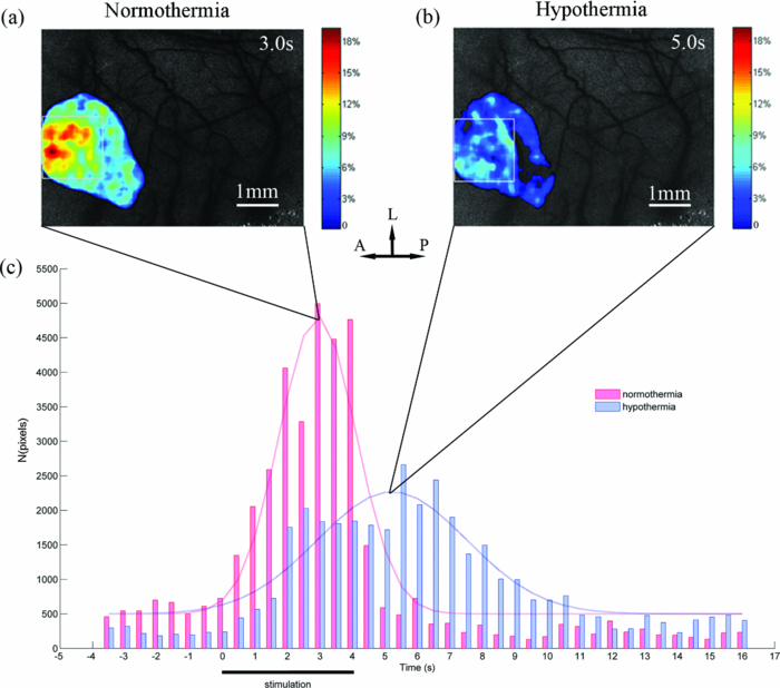

To detect the activation peaks, the TCA results [Fig. 3c] were fitted with the Gaussian function [i.e., N(t) in Eq. 5]

Table 2 lists the statistical results of the response peak and duration under different temperatures averaged across eight animals based on 10 trials in each subject. The time to response peak was around 2.6 ± 0.4 s post-stimulus onset at 37°C, which was significantly delayed to 5.2 ± 1.2 s at 32°C (P < 0.05) under hypothermia. Furthermore, the response duration under normothermia (2.6 ± 0.6 s) was significantly prolonged under hypothermia (5.3 ± 2.3 s) (P < 0.05).

Table 2

Spatial and temporal responses to 4 s hindpaw stimulation under normothermia and hypothermia (n = 8) in the aspect of relative CBF change. The time scale starts from the onset of a stimulus. (Data are presented as mean ± SD; *: paired t-test with hypothermia, P < 0.05.)

To show how much the CBF is correlated with the temperature, we present the scatter plots of the response peak [t_max, Fig. 4a] and response duration [R_d, Fig. 4b] under hypothermia versus normothermia for each animal. Linear regression analysis was performed to determine the correlation. The regression line in each plot was calculated according to y = ax, with y being the response values at hypothermia and x being the values at normothermia. Close correlations were observed between the responses (both t_max and R_d) under hypothermia and those under normothermia according to the correlation coefficients (t_max: r = 0.71; R_d: r = 0.82) with very similar slopes (t_max: s = 1.9271; R_d: s = 2.0955).

Fig. 4

Scatter plots showing the correlation of the (a) response peak (t_max) and (b) response duration (R_d) between normothermic and hypothermic stages. The best-fit line and correlation coefficient (R²) values represent the results of the linear regression analysis.

3.3.

Effects of Temperature on Spatial Activation

The OTCA method does not directly provide the spatial details of the cortical response. To investigate the spatial properties of the brain activation under hypothermia, a ROI (150×150 pixels) window, which covered more than 60% of the pixels with CBF change above the half maximum of the response peak by OTCA, was defined. The activation area, i.e., pixels with CBF above the half maximum within the ROI,³⁰ was used to quantify the CBF response.

Figure 3 illustrates the CBF change at t_max under normothermia [Fig. 3a] and hypothermia [Fig. 3b] for one animal. Table 2 shows the statistical results from eight animals, i.e., the activated area at t_max under normothermia is significantly larger than that under hypothermia (P < 0.05). There is also a statistically significant decrease in the peak relative CBF change ( [TeX:] $\Delta {\it CBF}_{t_{\max } } $ $\Delta {\mathit{CBF}}_{t_{\max }}$ ) from normothermia to hypothermia (P < 0.05).

Figure 5 shows the relationship between the [TeX:] $\Delta {\it CBF}_{t_{\max } } $ $\Delta {\mathit{CBF}}_{t_{\max }}$ under normothermia and that under hypothermia. An approximately linear correlation is observed for [TeX:] $\Delta {\it CBF}_{t_{\max } } $ $\Delta {\mathit{CBF}}_{t_{\max }}$ between two temperatures (r = 0.56).

Fig. 5

Scatter plots showing the correlation of the peak relative CBF change ( [TeX:] $\Delta {\it CBF}_{t_{\max } } $ $\Delta {\mathit{CBF}}_{t_{\max }}$ ) between normothermic and hypothermic stages. The best-fit line and correlation coefficient (R²) values represent the results of the linear regression analysis.

Taking advantage of the high spatial resolution of LSI, we were able to find the different blood flow changes in a rat's primary somatosensory cortex through hindpaw stimulation in different vessels from six rats with distinguishable vasculature (Fig. 6). The CBF changes in the venules (ROI C in Fig. 6) were less prominent than those in the capillary bed and arteriolar vessels (ROI B in Fig. 6), in accordance with the different hemoglobin dynamics in the arterioles, capillaries, and venules.³¹ The arterioles and venules were manually segmented by the anatomical features.

4.1.

Temporal Characteristics of Functional Activation

Under hypothermia, a significant delay of response was observed (P < 0.05), and the CBF recovered to the normal level (P < 0.05) more slowly. Under normothermia, CBF started to increase at ∼1 s and reached the peak at 2.6 ± 0.4 s after the stimulation onset, consistent with the reported hemodynamic changes during both forepaw³² and hindpaw³³ stimulations in rats by LDF and LSI, respectively. In modeling the stimuli-induced hemodynamic responses, the Gaussian function has been proven to be a more natural and flexible mathematical model than the Poisson or Gamma function.³⁴ It fits well with the data from optical intrinsic imaging and fMRI, especially in characterizing the time delay between the hemodynamic response and neural activities.^{34, 35} The correlation coefficients of the Gaussian fitting of our TCA data were compared between hypothermia and normothermia (0.9511 versus 0.9269), implying that the hemodynamic response still maintains the same temporal statistic model under hypothermia. The slower neuronal response under hypothermia may be caused by the suppression of the conduction in the peripheral nerve and spinal pathways³⁶ under low temperature. Thus, it increases the latencies and prolongs the durations of the excitatory postsynaptic potentials evoked by electrical stimulation.³⁷ The molecular mechanism of such delayed and prolonged response under hypothermia is probably related to the decreased release of neurotransmitters such as glutamate.²

4.2.

Spatial Characteristics of Functional Activation

Another interesting question is whether hypothermia could alter the activity-induced neurovascular or neurometabolic coupling. Our LSI results show that both the activation area and [TeX:] $\Delta {\it CBF}_{t_{\max } } $ $\Delta {\mathit{CBF}}_{t_{\max }}$ , in response to the functional hindpaw stimulation, were significantly reduced under hypothermia (P < 0.05). However, previous results from Royl ³⁸ show only the magnitude, and not the temporal features (i.e., latency and duration), of the relative CBF change under hypothermia that could have been caused by the limited spatial resolution of LDF. Fixed ROI chosen by traditional LDF would bias the relative CBF change because of the heterogeneous vasculature. OTCA solves this problem by defining the ROI dependent on the response results, which, therefore, provides higher spatiotemporal resolution of the functional representation of the CBF change without prior assumptions or knowledge on the spatiotemporal patterns of cortical activations. Note that the temporal profile of our CBF change by LSI is more consistent with Royl's finding on the electrophysiological response to somatosensory stimulation during hypothermia, i.e., the decreased amplitude and delayed peak time of somatosensory evoked potential (SEP), than the CBF results by the LDF method.³⁸ Combining the results with other electroencephalogram (EEG) findings, e.g., a decrease in EEG amplitude and a shift of EEG waves to lower frequencies under hypothermia conditions,³⁹ we can conclude that the neurovascular coupling is preserved during moderate hypothermia to some extent.

Most biological processes governing neuronal activity have a temperature coefficient (Q₁₀) between 2 and 3.³⁷ Q₁₀ is calculated as follows:

Furthermore, the reduced activation area and relative CBF change under hypothermia may imply that a smaller number of neurons are involved in functional activation. Nevertheless, considering the prolonged response duration under hypothermia, the total energy demand under hypothermia may not change compared with that under normothermia.

The spatial pattern of the vascular hemodynamic response is closely related to the neuronal function. So far, capillary responses to somatosensory stimulus have not been fully understood. Taking advantage of the high spatial resolution of LSI, we were able to investigate the hemodynamic response to somatosensory stimulus in a specific vascular compartment. Compared with the CBF changes in venules, the changes in arterioles and capillaries are more prominent. Such a different CBF response in the arterioles and capillaries could be explained by the received vasodilatory signals in the receptors on capillaries (or capillary dilatation), which then propagate along the vessels to the upstream arteriolar smooth muscle to regulate the blood flow to the neuropil.^{42, 43, 44} Therefore, our results suggest that large venules should be avoided when LDF is used to measure the activity-dependent CBF changes.

4.3.

Effects of Anesthetics

Like most studies on hypothermia, the animals in this study had to be anesthetized throughout the experiments, which could not prevent anesthesia-induced hypothermic hypometabolism. Anesthesia is also unavoidable in clinical hypothermic therapeutics. CBF can be decreased by pentobarbital, according to experimental and clinical studies,⁴⁵ although such pentobarbital-induced reduction of CBF is homogeneous.⁴⁶ The extent to which the accumulation of anesthetics can influence the response of CBF under functional stimulation is still unclear. Although no direct evidence exists to prove that the stimulus-induced CBF change is steady during anesthesia, in a study on rats on the effect of anesthetics on functional metabolic coupling in somatosensory stimulation, the regional cerebral metabolic rate of glucose is preserved under pentobarbital anesthesia.⁴⁷ In addition, the results of Royl ³⁸ did not show significant changes in SEP or CMRO₂ under functional stimulation during 3 h of normothermia following the same anesthesia protocols. Nevertheless, a stable anesthesia during the experiment is definitely helpful.