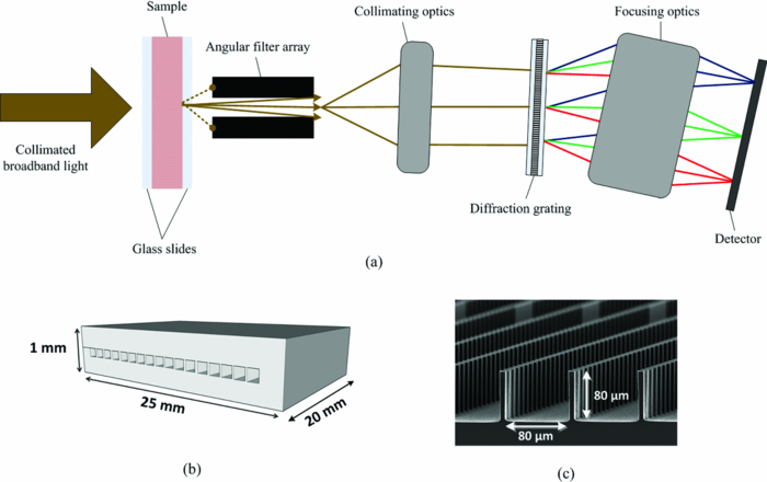
1.

Introduction

Hyperspectral imaging is a nondestructive optical analysis technique that integrates conventional spectroscopy and imaging to attain both spatial and spectral information from an object. Although hyperspectral imaging was primarily developed for remote sensing applications,¹ it has been implemented for other applications such as nondestructive thin tissue margin analysis.² Hyperspectral images are made up of at least 50 continuous wavebands for each spatial position of the target studied.^{3, 4} Consequently, each spatial pixel in a hyperspectral image contains a spectrum. The resulting spectral data adds another dimension to the two-dimensional (2D) spatial map resulting in a three-dimensional (3D) data cube. The spectral information can be used in many cases to identify the type of material represented by the pixel. When implemented with biological specimens, the technique can be used to identify tissues by type without the staining processes commonly used in histological protocols.^{5, 6}

Transillumination hyperspectral imaging is potentially applicable to the detection of internal optical contrast abnormalities for tissue samples < 0.5-mm thick. For instance, hyperspectral imaging shows potential for identifying margins of breast tumors intraoperatively during breast conserving surgery by identifying differences in optical contrast.⁶ In breast-conserving surgery, the objective is to excise the entire tumor while leaving normal tissue intact. Presently, the positive margin is only identified several days after surgery, after detailed histopathological examination of the excised tissue margins. In cases where tumor tissue is not completely removed after resection (with recurrence rate up to 20%),⁷ a second surgery may be required. Consequently, additional hospital resources and increased risk of patient morbidity becomes inevitable. As a result, it is crucial to accurately define the margins of the tumor intraoperatively.

Optical transillumination imaging of intrinsic optical contrast with sub-millimeter resolution for tissue specimens thicker than 1 mm is difficult due to the dominating contribution from optical scatter and the subsequent complex analysis of spectroscopic data. For this reason, many recent works have used either thin tissue slices or reflection-based measurements such as terahertz pulsed spectroscopy,⁸ optical coherence tomography,⁹ or Raman spectroscopy.¹⁰

In this paper, we present an innovative hyperspectral optical imaging technology called angular domain spectroscopic imaging (ADSI) that retains sub-millimeter spatial resolution as well as high spectral resolution through tissue specimens up to 3-mm thick. ADSI employs an array of microchannels to perform angular filtering of light that traverses a turbid sample. Angular filtration enables the rejection of scattered light at moderate levels of scattering (i.e., up to 20 mean free paths) that would normally corrupt spectral measurements. We hypothesized that the improved spectral data obtained with ADSI could provide a means to identify tissues from thicker tissue specimens while retaining sub-millimeter spatial resolution. Our objective was to evaluate the capabilities of an ADSI system by scanning tissue-mimicking phantoms as well as tissue samples from a tumor-bearing mouse to investigate the feasibility of tumor margin mapping by ADSI in freshly excised tissue.

2.

Materials and Methods

2.1.

ADSI Principle

The ADSI method is based on angular domain imaging (ADI), which has been shown to be adaptable to transmission, reflection, fluorescence, and time-domain approaches. ^{11, 12, 13, 14, 15, 16, 17} ADI employs parallel microchannels, which act as an angular filter array (AFA) with a small acceptance angle as shown in Fig. 1. By setting an appropriate and small acceptance angle, ballistic and quasiballistic photons from a collimated beam can be accepted by the filter, while scattered photons with exit angles outside the acceptance angle of the AFA are rejected [Fig. 1a]. In a related earlier analysis,¹⁸ Monte Carlo simulation results confirmed that the angularly-filtered photons emitted by the AFA are highly correlated to photons that travel the shortest path through a turbid medium (e.g., ballistic and quasiballistic photons). The simulation results also verified the image improvement with an angular filter and determined the resolution limitations. In ADSI, the AFA is combined with a “pushbroom” imaging spectrometer. The AFA is inserted after the sample and aligned with the spectrometer slit. The filtered photons accepted by the AFA are transferred to the dispersive element (such as a diffraction grating) and transformed into a two-dimensional image on a camera (one spatial axis and one spectral axis). The sample is then step-scanned in relation to the AFA and the 2D image capture is repeated. Repeated step-scanning with image capture results in a hyperspectral data cube that contains transmission spectra for a 2D rectangular grid of pixels representative of the spatial locations on the sample.

Fig. 1

(a) Schematic of ADSI principle (side view). (b) 3D schematic of a angular filter array (not to scale; smaller number of channels shown for clarity). (c) SEM picture of the bottom plate of an AFA where channels are located (flat top plate not shown for clarity).

2.2.

ADSI System Setup

The ADSI system was constructed from a halogen light source (100 W), collimation optics, an AFA, and an imaging spectrometer (P&P Optica Inc., Kitchener, Canada) as shown in Fig. 2. Light from the halogen lamp (from series Q lamp housing, model 60000, Oriel instruments, Stratfort, Connecticut) was first spectrally filtered to the red and near-infrared (NIR) region (650 to 950 nm). Spectral filtration was performed with Schott glass (long pass filter 645 nm, part no. 65.1365, Rolyn Optics Co., Covina, California), as well as a near-infrared shortpass filter (950 nm, 950FL07–50S, LOT-Oriel GmbH, Germany). The emitted light from the halogen lamp was focused using two condenser lenses. A pinhole with a diameter of 1 mm was used in combination with a NIR doublet spherical lens (ACH-NIR 25×50, Edmond Optics, New Jersey) with a focal length of 50 mm. A 15° holographic diffuser was placed before the pinhole to enhance the uniformity of the point source produced by the pinhole. The pinhole and lens system provided a collimated beam with an angular deviation of ∼1.15 deg. Since the AFA had a wide (horizontal), but short (height) field of view (20 mm × 80 μm), the collimated circular beam (∼2 cm in diameter) was shaped by placing a horizontal slit 2.5 mm in height in front of the sample to better match the illumination area to the AFA.

Fig. 2

Angular domain hyperspectral imaging diagram in transillumination mode: (a) top view, (b) side view.

The AFA was fabricated using silicon bulk micromachining used for fabrication of MEMS devices. The AFA consisted of 200 microchannels distributed as a linear array [see Fig. 1b and Fig. 1c]. Each channel had an 80 × 80 μm aperture, 20 μm channel wall thickness, and a channel length of 2 cm. Each microchannel provided acceptance angles of 0.23 deg from side-to-side and 0.32 deg from corner-to-corner. In order to minimize the intrachannel reflections, which could act as a source of background bias in the ADSI scans, the channel side walls were patterned with vertical ridges 2.5 μm in amplitude (>2 times the wavelength) at a periodicity of 20 μm [see Fig. 1c]. Fabrication details and complete analysis on the aspect ratio optimization and channel wall reflection effects on image contrast have been presented elsewhere.¹⁵ The AFA was positioned on a 6 deg of freedom jig to enable proper alignment with the incident collimated beam and the spectrometer.

The spectrometer design was based on a volume phase holographic transmission grating combined with refractive optics.¹⁹ A back-thinned CCD area image sensor was used (Hamamatsu Photonics K.K., Japan). The CCD had 2048 × 506 active pixels with an active area of 24.5 × 6.0 mm (square pixels each with an area of 12 × 12 μm). In this particular design, each pixel represented 12 μm in the spatial direction (each column) and 0.6 nm in the spectral direction (each row). Therefore, the total wavelength bandwidth of the CCD was 506 pixels × 0.6 nm/pixel = 303.6 nm and the total spatial width of the CCD was 24.576 mm. However, only 20 mm of the slit width of the imaging spectrometer was utilized due to the width of the AFA. The grating block was optimized for the spectral range of 650 to 950 nm. The input optics block of the spectrometer had an effective f-number of F/3.

Similar to conventional pushbroom spectrometers, the one-dimensional linear nature of the AFA allowed for one horizontal line to be imaged at a given time by the imaging spectrometer. The spectrum of each pixel was recorded into the corresponding column on the CCD. The height of the vertical step size was 100 μm, equal to the horizontal sample rate (AFA microchannel spacing), and so the sample was raised incrementally and scanned sequentially through different positions to image a large area. The sample was placed on a computer-controlled vertical z-axis stage between the output of the beam shaping system and the AFA. More detail on the scanning procedure has been described elsewhere.^{20, 21} Repeated ADSI scans at a sequential series of sample heights provided a 3D data cube of the sample. Fig. 3a shows the 2D spatial mapping of L-shape resolution targets (aluminum film as a reflective target on a glass slide) with various sizes (line and spacing thickness: 150, 200, 300, and 400 μm). As the spacing between each microchannel was about 100 μm, we expected to resolve L-shape targets with line thicknesses greater than 200 μm. However, the system spatial resolution was expected to degrade when imaging through turbid media, and even greater degradation was expected in real biological tissue due to high scattering heterogeneity.

Fig. 3

(a) ADSI scan (700 nm) of L-shape resolution targets in a nonscattering medium. (b) 3D CAD model of the mold used to prepare phantoms. (c) Schematic of a tissue-mimicking phantom. (d) Total attenuation (OD) spectra of ICG in 1% agarose/water solution in a 1 cm optical cuvette. (e) Total attenuation (OD) spectra of Intralipid™ in 2% agarose/water solution in a 1 cm optical cuvette.

3.

Results and Discussion

We calibrated and performed ADSI tests on a tissue-mimicking phantom and were able to resolve contrast targets at a variety of depths. Fig. 4a shows the projection image of the prepared phantom with 0.5% Intralipid™ and targets doped with ICG at 10 μM (left column) and 15 μM (right column) at three depths (rows). The images were assembled from 256 scan steps with step size of 100 μM, which set the vertical spatial resolution to resolve a line and space thickness of 200 μM. Since the spacing of the micro-channels was about 100 μM, we summed pixels horizontally (across each row) in groups of 8, which equated to 8 × 12 μM = 96 μM. The total area of the scan shown in Fig. 4a was 16.8 mm × 25.6 mm. The best image contrast in Fig. 4a was achieved at a wavelength of 840 nm. Image contrast degradation was expected to be much less dramatic compared with a conventional lens-based imaging system, since it is known that the AFA captures informative photons for projection image creation. The contrast is mainly due to quasi-ballistic/ballistic photons rather than scattered photons, which implies that identical targets at different depths should provide the same image contrast at a given sample thickness. However, leakage of scattered light through the AFA led to differences in image contrast for targets at different depths. This was highlighted by the differences in image contrast for the targets at different depths in Fig. 4a, where the image contrast decreased as the depth of the target increased. The effect of background scattered light due to leakage through the AFA has been discussed extensively in previous work.^{16, 17}

Fig. 4b displays artifact-corrected transmission spectra representative of Fig. 4a at four different regions of interest. The regions were selected from the central areas of the three 15 μM ICG targets. The spectral transmission of the reference point corresponding to the center point of the 15 μM ICG target at the shallowest depth (1 mm) is presented with solid black lines [Fig. 4b]. Another region corresponding to the body of the phantom (i.e., a region absent of ICG absorbing targets) was also selected and displayed for reference (green curves). Although fresh ICG solution in water showed the highest absorption at ∼780 nm [Fig. 3d], the transmission spectra of ICG targets in the phantom [Fig. 4b] demonstrated a redshift of the peak absorption wavelength. This was due to the presence of Intralipid™ within each ICG target as well as Intralipid™ through the background optical path. Intralipid™ has lower absorption at longer wavelengths [Fig. 3e], which leads to greater light transmission and the appearance of a redshift in the ICG spectrum compared to ICG in a nonscattering medium.

Fig. 4c and Fig. 4d present the correlation maps of a phantom based on a designated reference point for a suboptimal and optimal threshold level, respectively. In these particular examples, the reference point was located at the center of 15 μM ICG target at the shallowest depth (1 mm). The correlation map of the phantom shown in Fig. 4c was thresholded at a correlation value of 0.5 while the correlation map of the phantom in Fig. 4d was thresholded at a correlation value of 0.6. Throughout the phantom studies, the correlation value was based on the transmission intensity between 750 and 870 nm, which was found to be the optimal spectral range. The optimal correlation threshold level is highly dependent on the similarity of the reference spectral signature compared to the spectra at other locations in the image, which is highly related to the distinctiveness of the embedded abnormality. For our tissue-mimicking phantom analysis, the optimal correlation threshold level was empirically selected to minimize the background signal, but maintain the size and shape of the spherical targets.

The reference spectral signature for the spectral correlation analysis was also extracted from the first derivative of the transmission spectra within the 3D data cube. Fig. 5a presents the first derivative of the transmission spectra shown in Fig. 4b for the 15 μM ICG target at three depth positions as well as the background region. As shown in Fig. 5a, the first derivative of the transmission spectra of the target was less dependent on depth compared to the zero order transmission spectra [Fig. 4b]. Therefore, in the first order correlation mapping, the optimal threshold level selected for the zero order analysis (R = 0.6) was not expected to be a suitable threshold for the first order correlation mapping. Instead, the similarity in the first order transmission spectra at different depths suggested that a higher threshold level was more suitable. When the first order correlation map was computed with a sub-optimal threshold [R = 0.6, Fig. 5b], a background signal was apparent and the edges of the targets were less defined, especially for the deeper targets. The first order correlation map computed with a higher threshold level [R = 0.8, Fig. 5c] had almost no background signal and the targets at all depths were well resolved.

Comparison of the correlation maps extracted from zero and first order transmission spectra (Fig. 4 and Fig. 5), suggested that the first derivative provided a more robust spectral signature against the effects of scattering and depth of the targets. This result was observed for both the sub-optimal and optimal threshold selections for the first order correlation mappings in Fig. 5b and Fig. 5c. This was apparent by the better overlap of first order spectra outside of the absorbance band of ICG for the targets at different depths, where the zero order spectra were significantly offset from one another. Although spectroscopic etaloning appeared to be corrected in zero order transmission spectra, the first order spectra for targets at different depths contained periodic patterns, which were likely due to the effects of spectroscopic etaloning [Fig. 5a] enhanced by numerical differentiation.

Fig. 4

(a) Angular domain spectroscopic images of a 7-mm thick gel phantom with 0.5% Intralipid™ and 3-mm spherical targets doped with 10 and 15 μM ICG at 7 wavelength bands (phantom #1). (b) Transmission spectra of the center position of three spherical targets (15 μM ICG) versus the background spectra (spatial and spectral artifacts removed). (c) Correlation map with sub-optimal threshold level computed from the ADSI image, where the black curve in (b) was used as the reference. (d) Correlation map with optimal threshold level computed from the ADSI image, where the black curve in (b) was used as the reference.

Fig. 5

(a) First derivative of the transmission spectra presented in angular domain spectroscopic images of a 7-mm thick gel phantom with 0.5% Intralipid™ and targets doped with 15 μM ICG (phantom #1). (b) Correlation map of phantom with sub-optimal threshold level using first derivative transmission spectra of the center position of spherical target (15 μM ICG, 1 mm depth, at lowest row) as a reference spectral signature. (c) Correlation map of phantom with optimal threshold level using first derivative transmission spectra of the center position of spherical target (15 μM ICG, 1 mm depth) as a reference spectral signature.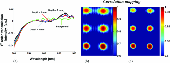

In order to analyze the sensitivity of the ADSI system, we tested another phantom with the same geometrical structure, but with targets at different scattering and absorption levels. The second phantom contained 0.4% Intralipid™ as a scattering background, which has an approximately 20% lower scattering coefficient compared to phantom #1. In phantom #2, the targets were doped with 1 and 5 μM ICG in the left and right columns, respectively. The absorption coefficient for 5 μM ICG in second phantom was approximately 67% less than phantom #1 (15 μM ICG). While the reduced scattering level in phantom #2, compared to phantom #1, suggested that more quasiballistic light was available for detection. However, the significantly reduced absorption in the targets was expected to push the ADSI system to its detection limit. Fig. 6a and Fig. 6b show the zero order transmission spectra of the 5 and 1 μM ICG targets versus background. Fig. 6c and Fig. 6d present the first order transmission spectra for the 5 and 1 μM ICG targets versus background. Fig. 6e and Fig. 6f present the correlation maps computed with the zero and first order spectra at a suboptimal (left panel) and an optimal (right panel) threshold level. The region corresponding to the 5 μM ICG target at shallowest depth (1 mm) was used as the spectral signature reference. We observed a similar improvement in visibility of the targets using first derivative spectral transmission data in the correlation analysis [see Fig. 6f] over zero order transmission data [see Fig. 6e] when compared to the ADSI results from phantom #1.

Fig. 6

Spectral analysis of the ADSI scan for phantom #2. (a) Transmission spectra of the 5 μM ICG doped target at three different depths. (b) Transmission spectra of the 1 μM ICG doped target at three different depths. (c) First derivative of the spectral transmission shown in (a). (d) First derivative of the spectral transmission shown in (b). (e) Correlation map computed using a sub-optimal threshold level (left panel) and an optimal threshold level (right panel) of phantom #2 based on zero order spectra using the center point of the 5 μM ICG target at the lowest row as a reference point (1 mm depth). (f) Correlation map computed using a sub-optimal threshold level (left panel) and an optimal threshold level (right panel) of phantom #2 based on first order spectra and the center point of the 5 μM ICG target at the lowest row (1 mm depth) as the reference point.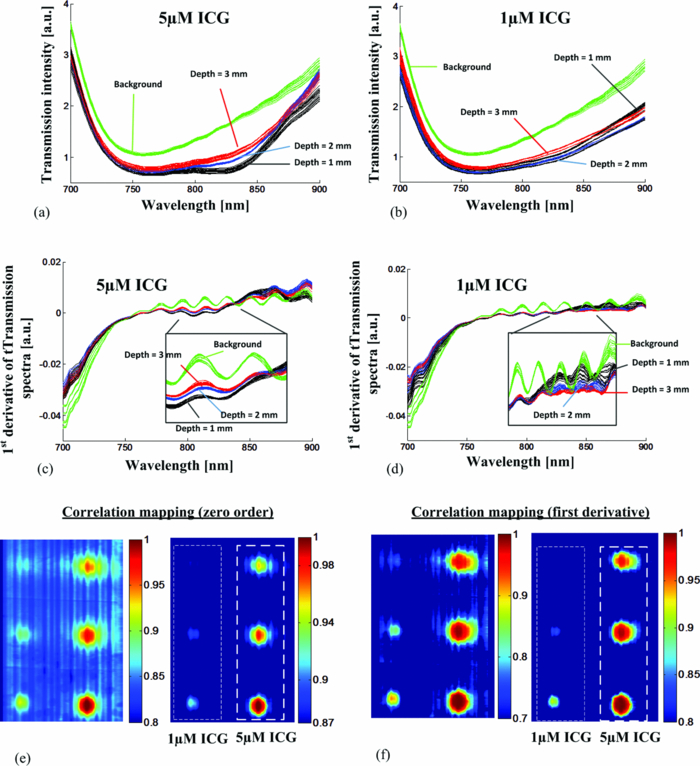

The optimal correlation threshold using the zero order transmission correlation mapping in phantom #2 (R = 0.87) was higher than the threshold selected for the corresponding correlation mapping in phantom #1. This was due to the higher similarity in the spectral transmission intensity for the three targets compared to the background signal for phantom #2. When the correlation mapping for phantom #2 was displayed with the sub-optimal correlation threshold (R = 0.8), a large background signal was apparent in the image. In contrast, the optimal correlation threshold for the first derivative correlation mapping was the same for phantom #1 and phantom #2 (R = 0.8). This result suggested that the first derivative correlation mapping was more robust against target absorption and scattering variation.

Interpretation of the correlation mappings of the first order transmission intensity for phantom #1 and phantom #2 suggested that there was a tradeoff between the absorption coefficient of the embedded targets versus the scattering coefficient from the surrounding material, which affected the detection limit of ADSI. For instance, the optimal correlation threshold in phantom # 1 and #2 was about R = 0.8, even though each phantom had different scattering properties and different target concentrations. It is generally known from ADI experiments that perfect absorbers can be detected at the highest scattering background (in our case up to 1% Intralipid™ with 7 mm phantom thickness),¹⁵ and that the scattering limit will decrease as the optical absorption of the target decreases. This explains, in part, why the 1 μM ICG targets were barely visible at a correlation threshold of 0.8 with the reference signal taken from a region within the 5 μM ICG target.

For phantom #2, the 1 μM ICG target was detected at the shallower depths (1 and 2 mm), in both the zero order and first derivative correlation mappings at sub-optimal and optimal correlation thresholds. The 1 μM target was not observed at the deepest position (3 mm) for the correlation mappings with optimal correlation threshold. The 1 μM target was only detectable at the deepest position with a sub-optimal correlation threshold, which lowered the threshold of detectability at the expense of reduced background suppression. For all of the correlation mappings, the size and the signal of the 1 μM target were significantly reduced. This was expected for two reasons. First, the 5 μM target was used as a reference signal for the correlation computation. Second, the shape of the absorption spectra of 5 μM ICG was different from 1 μM ICG [Fig. 3d], which would lead to further reductions in the computed correlation values.

As shown in Fig. 7a and Fig. 7b, the ADSI system was tested on a slice of tumor tissue (3-mm thick) dissected from an SCCVII tumor bearing nu/nu mouse. Fig. 7b shows the front and back side of tissue sample sandwiched between two glass slides. The front side of the tissue sample was masked with black tape in order to reject the nonscattered illumination from the source (which potentially could saturate the CCD). The sample included regions of muscle, bone, fat, and blood. Fig. 7c presents the transmission spectra of selected regions known to be muscle or tumor tissue. The significant drop in contrast in the masked and bone regions did not provide enough dynamic range for spectral analysis. The transmitted light intensity projected through the tissue sample resulted in an image with a gray-scale intensity map that was affected by several factors including spatially-dependent illumination intensity variations, AFA geometrical arrangement, tissue thickness, and tissue composition. Each of these factors could potentially affect the image contrast in a manner that depended on wavelength and spatial position. Therefore, in order to isolate the informative part of the spectral signal variation due to tissue composition, spectral normalization, and calibration procedures were implemented.

Fig. 7

(a) Cross section diagram of tissue sample for ADSI testing. (b) Color photographs of mouse tumor tissue sandwiched between two glasses slides. The opening due to the black mask that was used for transmission imaging is marked by the yellow dashed line. The black line (left panel) indicates the location of bone embedded in the tissue. (c) Normalized spectra from regions of tumor and muscle tissue [as indicated in (b)]. (d) Correlation map of data cube based on reference spectral signature related to the muscle tissue. (e) Correlation map of data cube based on reference spectral signature related to the tumor tissue.

To account for CCD saturation effects during the capture of the illumination source, a neutral density filter (OD4) was used to reduce the intensity of the source in place of the sample. Fig. 7d and Fig. 7e show the spectral correlation maps of the sliced tissue sample shown in Fig. 7b. Fig. 7d shows the correlation map for the tissue specimen, where the reference region was taken from the muscle tissue region (indicated by tagged square). Fig. 7e shows the correlation map of the tissue specimen, where the reference point was positioned within the tumor region (tagged square). The correlation threshold level was highly dependent on the similarity of reference signal to the other areas. Hence, the optimal threshold level was found to be R = 0.6 for the muscle tissue correlation map, while the optimal threshold increased to R = 0.99 when the tumor area was used as a reference signal.

The correlation analysis in the tissue sample revealed that the optimal threshold level was highly dependent on the differences between the transmission spectra of the reference tissue type compared to the others. For instance, muscle tissue provided a faster change in attenuation at longer wavelengths compared to fat, fibrous, and tumor tissues. Therefore, by setting R = 0.6 the muscle tissue regions were easily separated from other tissue types. However, distinguishing tumor regions from other tissues was more challenging. By selecting the reference transmission spectra from a tumor region, the threshold level had to be increased up to R = 0.99 to clearly visualize the tumor tissue margin. This was mainly due to the similarity of transmission spectra for tumor and fibrous tissue in the near-infrared region.

One method to improve the differentiation of tumor from surrounding tissue may be to implement ADSI for sliced fresh tissue in the visible range, where there are more numerous spectral differences between tissue types. Using light in the visible region (500 to 750 nm) would significantly decrease the spectral etaloning effects observed. Reduction or elimination of spectral etaloning would reduce the need for artifact correction post-processing steps and the overall time to image display. The drawback from using light in the visible region is the expectation of increased scatter, which could be mitigated by interrogating thinner tissue slices (∼1 mm).

Correlation mapping of the tissue-mimicking phantoms proved to be a useful algorithm for the identification of similarities in the spectral response from image regions of unknown composition compared to regions of a known composition (reference signal). However, in heterogeneous tissue samples, more than two significant spectral signatures are likely to be present and hence more complex post-processing algorithms are likely to be required. Principal component analysis (PCA) and linear discriminant analysis (LDA) are examples of algorithms that have been successfully employed to identify different tissue components in mass spectroscopy imaging,²⁷ Raman spectroscopy,^{28, 29} and FTIR spectroscopy.³⁰ Nonlinear techniques have been proposed as more robust alternatives to PCA and LDA for classification of tissue types from image data.³¹ With further advances in ADSI instrumentation (more rapid image capture, higher dynamic range, and use of visible light) detailed testing of more robust tissue classification schemes that utilize ADSI data will be justified.

4.

Conclusion

An ADSI system was constructed by adapting an ADI system with an imaging spectrometer. The system was experimentally tested using 7-mm thick tissue-mimicking phantoms with embedded ICG doped spherical targets as well as 3-mm thick tissue samples dissected from a nu/nu mouse. The imaging system employed a silicon micromachined angular filter array, which had high angular selectivity for photons exiting the tissue sample. Spectral differences between targets and background in phantom studies, as well as tumor and muscle in the murine specimen, were resolvable with ADSI, which suggested that the technique has potential for the characterization of thicker tissue samples compared to conventional histopathological analysis of ex vivo tissue samples.