2.1.1.

Subjects

Seven subjects that were recruited in our laboratory (five male and two female with normal or corrected-to-normal vision and no reported history of neurological problems; age 27 to 37) volunteered for the behavioral experiment, and five of them (three male and two female; age 33 to 37) participated in the NIRS experiment. Two of them were the authors. The other subjects were familiar in general with psychophysical and NIRS experiments but not informed of the purpose of these particular experiments. All the subjects provided written informed consent. All measurements were conducted with the approval of the Ethics Committee of Hitachi, Ltd.

2.1.2.

Change-detection task

A task designed by Beck ¹¹ was used for both the behavioral and NIRS experiments. A single trial of this task consisted of two subtasks—a character task and a face task—and the subjects were instructed to respond to both of the subtasks. The time line of stimulus presentation and subject's responses is shown in Fig. 1. First, a fixation cross appeared at the center of a display on which subjects were instructed to fixate during the trial. A screen with two faces, one on the right and another on the left (each 2.0 deg from the fixation cross), was then shown for 500 ms. At the same time, two alphabet strings composed of three characters were shown (2.4 deg above and below the fixation cross). The face images and character strings subtended 3.2 × 3.7 and 1.8 × 1.0 deg, respectively. Four facial images of middle-aged men wearing glasses, adopted from a face-image database,⁵⁹ were used (see upper-right inset in Fig. 1). Then, a uniform gray blank screen was interleaved for 500 ms. The screen with faces and character strings and the gray screen were repeated four times. The subjects were seated ∼30 cm in front of the computer display with their heads stabilized on a chin rest and were instructed to keep fixating at the fixation cross. While the screen was flickering, the subjects were asked to report if a target character (in this case X) was contained either in the top or bottom of the screen by using the key pad of an external keyboard (pressing “7” for an X present in top, “0” for an X present at bottom, or no key press indicating the absence of an X). This procedure was referred to as the character task. The target character appeared in one-third of the runs either at the top or bottom at one time.

Fig. 1

Schematics of the time course of a single trial of the change-detection task. The upper-right inset shows the four faces used in the experiment.⁵⁹ In a single trial, the subjects were instructed to respond to the face task for four times and to the face task once at the end of a trial.

At the end of each trial run, a question mark appearing at the center of the screen for 1000 ms prompted subjects to report if there was a change in the face stimuli during the character task (pressing “0” for no change or “8” for change). This subtask was referred to as the face task. The subject had three chances to notice a change of the face stimuli. A single-trial of the change-detection task run took 5.0 s. Because the attentional resources of the visual system were divided into the two tasks described above, occasional failure to detect face changes was expected. In-house Matlab codes on a Windows-based laptop computer were used to present the face and character-string stimuli and to record subjects’ responses for later off-line analysis.

The face stimuli were changed in two-thirds of all trials. These trials are hereafter referred to as the face-change trials in which either the left stimulus or the right stimulus was changed at equal frequency [referred to as left-change (LC) or right-change (RC) trials, respectively]. In the remaining one-third of the entire trials, the face stimuli were not changed [no change (NC) trials]. The NC trials were included to avoid the risk that subjects might falsely report a change without paying attention to the face stimuli. The sequence LC, RC, and NC trials was randomized session by session so that the subjects could not memorize it from previous sessions with a constraint of equal frequencies. In some change trials, the subjects correctly reported a change in the face stimuli (defined as successful trials), but in other change trials the subjects failed to report a change irrespective of the physical change (defined as unsuccessful trials). Subjects were instructed to report a change in the face task only when they were confident that a change occurred.

2.1.3.

Behavioral experiment

A behavioral experiment was conducted prior to the NIRS experiment described below. The purpose of this experiment was twofold, namely, to familiarize the subjects with this rather difficult change-detection task and to evaluate the task difficulty so as to invoke change blindness to some degree. One session consisted of 25 NC trials, 25 LC trials, and 25 RC trials (totally, 75 trials) and took ∼8 min. The intertrial interval was 1.0 s. Seven subjects attended three to seven sessions each (4.0 sessions on average). The subjects’ responses during the character task and the face task were recorded for later analysis. During this behavioral experiment, the experimenter closely watched the eye movements of subjects and instructed to keep fixating at the fixation cross whenever they broke their fixations.

2.1.4.

Near-infrared spectroscopy experiment

The same change-detection task as described above was used for the NIRS experiment, with a few modifications. First, the intertrial interval was taken randomly from 20 to 25 s so that the hemodynamic responses went back to the baseline level by the beginning of each trial.⁶⁰ Second, to minimize the physical burden and to conduct each session in a reasonable time, the total number of trials was limited to 30 (10 NC, 10 LC, and 10 RC trials). The 30 trials took ∼14 min, and the whole experimental duration, including NIRS preparation, took ∼30 min. No subjects reported any discomfort either during or after the experimental session.

An ETG-7000 (Hitachi Medical Co., Tokyo, Japan) was used for the NIRS measurements and was controlled by the same Windows-based computer used for the visual-stimulus presentation and response recording. Sixty probes (32 light-emitting optical fibers and 28 light-detecting optical fibers) were stabilized on the scalp by means of four probe-holder sheets, each of which had 15 probes. Each laser emitter and detector formed a pair that provided a recording channel, resulting in 88 channels in total (Fig. 2). Note that channels refer to cortical locations, located approximately at the midline of corresponding laser emitters and detectors that are located on the scalp.⁶¹ The probe-holder sheets were connected to each other with elastic bands. The landmarks of the nasion, inion, and the left and right tragus in the ear were identified for each subject, and the reference site C _z was determined from these four landmarks according to the international 10–20 method.⁶² The probe-holder sheets were arranged so that their center of mass was located at C _z. To map out the corresponding cortical locations, the actual three-dimensional positions of all probes were measured with a three-dimensional digitizer (ISOTRAK II, Polhemus Corporation, Colchester, Vermont) for two subjects. The three-dimensional locations of channels were derived as midpoints of the corresponding light-emitter/-detector pairs. These locations were first translated into MNI coordinates by using statistical spatial registration⁶³ and then into corresponding cortical areas by applying automatic anatomical labeling.⁶⁴

Fig. 2

Cortical locations of 88 channels measured by averaging data from two subjects.

2.2.1.

Behavioral data analysis

Correct responses and reaction times in the behavioral experiment, for both the character task and the face task, were counted. In a single trial of the character task, the subjects had to report the presence or absence of the target character X and its location in four consecutive screens. Responses were defined as successful when subjects correctly reported the location of the X when it was present and when subjects did not press any key when no X was present. Any other responses were regarded as unsuccessful. The correct-response ratio was computed by dividing the number of successful trials by the number of screens presented to subjects. The distribution of reaction times of successful responses when the subjects correctly reported the presence of an X was also computed.

For the face task, trials were defined as successful if subjects reported a change when there was a change in the face stimuli or if subjects reported no change when there was no change in the face stimuli. The correct-response ratio was defined as the ratio of successful trials to the number of trials. The correct-response ratio and the response times for the NC, LC, and RC trials were computed.

2.2.2.

Preprocessing of near-infrared spectroscopy data

All analysis procedures were performed offline. Oxy-hemoglobin-concentration signals were used for the analysis because they have been shown to have a high signal-to-noise ratio.⁶⁶ The NIRS signals were preprocessed as follows. First, to remove certain noises of extra-cortex origins, such as pulsations, a temporal moving average over 3.0-s duration was applied.^{67, 68} A third-order polynomial a ₀ + a ₁ t + a ₂ t ² + a ₃ t ³ was fitted to NIRS signals of an entire experimental session by the least-squares method, and this polynomial component was subtracted from the NIRS signals in order to remove global trends. This polynomial detrending was applied separately to all channels. This procedure ensured that the detrended NIRS signals had no drift components.

The subsequent classification analysis used NIRS signals from combinations of channels and required a considerable computational resource. Out of the entire 88 channels, those noisy channels were therefore excluded if their amplitudes exceeded 0.5. Channels whose power spectrum appeared to be white were also excluded according to the following criterion. Low-frequency components (<3.0 Hz) contain biologically relevant signals including hemodynamic changes, whereas high-frequency components (>3.0) can be regarded as biologically irrelevant noises. If the spectrum power of the high-frequency band is comparable to that of the low-frequency band in a NIRS channel, then biologically relevant signals in the low-frequency band are not to be detected due to high-frequency noise. In other words, the ratio of low- and high-frequency bands can be used as a measure of “whiteness.” A t-test was applied to determine whether the spectrum power of low- (0.01–0.5 Hz) and high-frequency bands (4.0–4.5 Hz) in each channel was statistically distinguishable (an indication that the channel's spectrum differed from a white spectrum). Channels were used for further analysis if the p-value computed in the t-test was smaller than an empirically determined threshold of 1 × 10⁻¹⁰, and were excluded otherwise. The threshold p-value was empirically determined by visual inspection of NIRS data in this study. A more objective criterion for determining a threshold value is being developed.

2.2.3.

Classification analysis by support-vector machine

There are a variety of machine-learning algorithms applied to classification of neuroimaging data. Some examples are minimum-distance classification,⁶⁹ Fisher's linear-discriminant analysis (LDA),⁷⁰ support-vector-machine (SVM) algorithms,⁷¹ and hidden Markov models.⁵² In this study, a support-vector-machine algorithm with a linear kernel⁷² was adopted for the binary classification problem.

To exploit the temporal resolution of NIRS, classification probabilities of successful and unsuccessful trials were computed in time steps of 0.1 s (Fig. 4). First, a combination of channels was chosen, NIRS signals were extracted from all face-change trials, and each subject's trial was labeled as being a change-detected (successful) or change-undetected (unsuccessful) trial [green and red lines, respectively, in Fig. 4a]. The signals were then averaged in a temporal window [blue-shaded areas in Fig. 4a] to give points in a multidimensional space [Fig. 4b]. The width of the temporal window was fixed at 3.0 s, and the onset of the temporal average was varied from −5.0 to 13.0 s in steps of 0.1 s (note that 0 s was defined as the onset of the task). The SVM classification algorithm was then applied to the points of the multidimensional space [Fig. 4b]. To evaluate how well the data points could be classified, twofold cross validation was used [Figs. 4c and 4d]. Approximately half of the data points were randomly selected as training data [green and red points in Fig. 4c], and the rest were preserved as test data [gray points in Fig. 4c]. An SVM decision boundary was computed using only the training data [blue dashed line in Fig. 4c]. The performance of the decision boundary was evaluated by applying it to the test data [green and red points in Fig. 4d] and by computing the probability that the test data were correctly classified>. (defined as classification probability). This cross-validation procedure [Figs. 4c and 4d] was repeated 30 times with randomly chosen test and trial data in order to compute the mean classification probability and its confidence intervals. This SVM classification was performed on a subject-by-subject basis; a decision boundary was determined from a subject's data and its performance was evaluated with the same subject's data.

Fig. 4

Schematic of classification analysis procedure. (a) A pair of NIRS signals recorded in change trials. Green and red lines depict signals in change-detected and change-undetected trials, respectively. The blue shaded area is an example of a temporal window in which the NIRS signals were averaged. (b) Two-dimensional map of temporally averaged NIRS signals obtained from the data in (a). (c) SVM classification applied to training data (a decision boundary indicated by blue dashed line) and (d) cross validation of the decision boundary using test data. These plots were created from actual experimental data. (Color online only.)

2.2.4.

Number of channels used for classification analysis

Before applying the classification procedure described earlier, it was necessary to determine how many dimensions or channels should be used. In general, there should be optimal dimensions for a classification problem. Small feature dimensions may not provide sufficient information for classifying the change-detected and change-undetected trials. On the other hand, large feature dimensions incur the risk of overfitting to training data. Too small or too large feature dimensions both result in poor performance of classification of the test data. Moreover, the number of possible combinations of features grows rapidly with an increasing number of feature dimensions; therefore, it is desirable to keep the feature dimension as small as possible to save the computational time needed for analysis. For the classification problem stated in Sec. 2.2.3, the performances of classification using single channels, pairs of channels, or triplets of channels were compared in terms of the test data of Subject 1. After the number of channels was determined, the same number of channels was used for the data of other subjects.

2.2.5.

Clustering analysis of temporal classification probabilities

To discover typical temporal profiles of classification probabilities, an unsupervised classification algorithm was applied to the classification probabilities computed by using the SVM method (as described in Sec. 2.2.4). The k-means clustering algorithm with a squared Euclidean distance was adopted as a similarity measure.⁷³ The number of clusters was adjusted by visual inspection.

3.2.1.

Optimal number of channels necessary for classification algorithm

To determine the optimal number of channels, the classification probabilities were evaluated by using single channels (60), channel pairs (₆₀ C ₂ = 1,770), and channel triplets (₆₀ C ₃ = 34,220) and the response data of Subject 1. The computation for these three cases took, respectively, 15 min, 7.2 h, and five days on a Windows-based computer (Intel Core2Duo, 3.0 GHz). Figure 6 summarizes 50 classification probabilities that varied significantly in their time courses for the three cases. Average values of maximum classification probabilities of the 50 combinations were 77% (SD 6.7%), 86% (SD 3.1%), and 87% (SD 2.1%). The classification probabilities in the channel-pair case were considerably improved compared to those in the single-channel case. In contrast, when channel triplets were used instead of the channel pairs, the classification probabilities changed little, indicating that the channel pairs were sufficient for classifying the successful from unsuccessful trials. Moreover, the exhaustive search using channel triplets was prohibitively time consuming for analyzing the data of multiple subjects. Accordingly, channel pairs were used for further analyses of the other subjects.

Fig. 6

Classification probabilities computed from (a) single channels, (b) channel pairs, and (c) channel triplets. The dashed lines indicate average values of maximum of all probabilities.

3.2.2.

Distribution of classification probabilities

Moment-by-moment classification probabilities were computed using all possible channel pairs for the four subjects. The temporal window was first fixed, and the population distributions of classification probabilities for possible channel pairs were investigated. The red histograms in Fig. 7 illustrate distributions of classification probabilities computed using all channel pairs for Subject 1 during the task period (0–3 s) [Fig. 7a] and 5 s after the task completion (10–13 s) [Fig. 7b]. The distribution in Fig. 7a had a mean of 51.6% and a standard deviation of 7.3%. In contrast, the distribution in Fig. 7b had a mean of 61.3% and a standard deviation of 10.1%. Figures 7c and 7d illustrate NIRS signals that show the maximum and 50% classification probabilities, respectively, in the distribution of Fig. 7b.

Fig. 7

Classification probabilities (red histograms) obtained by using the NIRS signals from all 1770 channel pairs (a) during task (0- and 3-s interval) and (b) after task completion (10- and 13-s interval). The blue histograms describe classification probabilities computed from surrogate data (i.e., randomly relabeled as successful and unsuccessful trials). Examples of NIRS signals, found in the posttrial distribution which: (c) gave 50% probability and (d) gave the highest probability. The blue dashed line in (d) indicates the decision boundary computed by an SVM algorithm. (Color online only.)

Note that the distributions computed using randomly relabeled, surrogate data [blue histograms in Figs. 7a and 7b] were highly peaked and did not change during and after the task. The differences between the histograms computed using the subjects’ response and surrogate data were statistically significant [Mann–Whitney U-test; p = 8.9 × 10⁻⁴ for Fig. 7a, and p = 6.2 × 10⁻¹²⁸ for Fig. 7b]. This analysis confirmed that the high values of posttrial classification could not be attributed to a statistical chance.

3.2.3.

Temporal profiles of classification probabilities

It was found that there were, generally, two types of temporal profiles, which we call postdictive and predictive. The postdictive type of temporal profile exhibited a plateau before and during the task period, a gradual increase on task completion, and a peak value ∼5 s after task completion. Figure 8a illustrates a representative probability profile computed from a channel pair (25, 33) of Subject 1 [for corresponding images of the NIRS signal, see Appendix (Fig. 11 and 1). By classifying the signals of this channel pair, it was possible to determine if this subject noticed a face change in the change trial that had just been finished. We interpreted that this temporal profile of classification probability reflected the success or failure of a trial.

Fig. 11

Snapshots of NIRS signals from t = −5.0 to t = 10.0 that were used to compute the probability in Fig. 8a. Horizontal and vertical axes in each image denote temporally averaged NIRS signals from channels 25 and 33, respectively. The pink shade indicates the task period. The blue dashed lines depicting the decision boundaries are included if the classification probability is >75%. (Color online only.)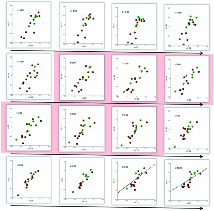

The predictive type of temporal profile was found in the case of Subject 2 [Fig. 8b]. The classification probability increased 3.0 s before task initiation, took a maximum value around the time of the task initiation, and decreased to approximately the correct response ratio [for corresponding snapshots of NIRS signal, see Appendix (Fig. 12 and 1)]. By classifying the signals of this channel pair, it was possible to predict whether the subject noticed a face chance immediately before the trial was completed. The signals from this channel pair were interpreted as predictive for the success or failure of a trial

Fig. 12

Images of NIRS signals used for Fig. 8b. Channels 4 and 32 were used for the horizontal and vertical axes. The pink shade indicates the task period. (Color online only.)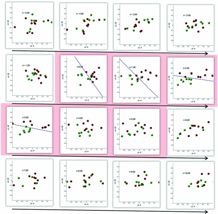

Video 1

NIRS signals and classification probabilities. (WMV, 4.9 MB)1

3.2.4.

Analysis of four subjects

We performed the same classification procedure exhaustively on all possible channel pairs (1770, 1596, 3828, and 2580 pairs from Subjects 1–4, respectively; see Table 1). Because the temporal dynamics of classification probabilities was the focus of interest, the 50 channel pairs that showed maximal amplitudes of classification probabilities (i.e., maximum probability – minimum probability in each temporal profile) were chosen. Figure 9 summarizes the results for Subjects 1 and 3. Classification probabilities in Fig. 9a (Subject 1) had postdictive temporal profiles that were similar to the one shown in Fig. 8a. The corresponding channel pairs from which the probabilities in Fig. 9a were computed are shown in Fig. 9b. We looked for the most informative channels, or hubs, which are defined as NIRS channels that most frequently appeared in the 50 channel pairs. Channel 33 (indicated by a blue circle) located in the left angular gyrus appeared in 32 channel pairs out of the total 50 channel pairs, contributing most to the postdicitive classification. The results for Subject 3 are summarized in Figs. 9c and 9d, exhibiting characteristics similar to those of Subject 1. The most informative channel was channel 35 (indicated by a blue circle), which was located in the left occipital area and appeared in 24 channel pairs. For both subjects, the pairs that contained channels in the left temporoparietal or occipital areas gave the higher values of classification probabilities, and the most informative channels tended to be paired with channels in the frontal lobe [Figs. 9b and 9d].

Fig. 9

(a) Temporal profiles of the classification probability computed using the NIRS signals of Subject 1. The pink-shaded area depicts the task period. The light blue line denotes the average values of all probabilities. (b) Channel pairs used to compute the probabilities shown in (a). The pairs are connected by light blue lines. The black filled circles describe the locations of the channels used for the analysis, and gray filled circles the locations of the channels that were excluded according to the criteria stated in Sec. 2. The numbers printed on the channels indicate the cortical location depicted in Fig. 2. (c) Temporal classification probabilities of Subject 3 and (d) the locations of the channels pairs. (Color online only.)

Figure 10a shows predictive temporal profiles of classification probabilities computed from 50 channel pairs of Subject 2. Most temporal profiles exhibited maximum values before the task completion, thereby predicting whether that subject would report the presence or absence of a face change. Pairs that contained channels in the right temporoparietal areas contributed to these high-classification probabilities [Fig. 10b]. Channel 20 (located at the right occipito-temporal junction), appearing in 34 pairs, was most informative for this predictive classification. Subjects 1–3 had either pre- or postdicitive temporal profiles only. Interestingly, Subject 4 had both pre- and postdicitive components [Fig. 10c]. Channel pairs that had posterior-parietal-lobe channels had contributed to both pre- and postdicitive classification [light blue and purple curves for postdictive and predictive classification, Fig. 10d]. Channel 32 (located in the posterior parietal area) appeared in 34 pairs and was most informative for postdictive classification (a blue circle), and channel 36 (located in the postcentral area) appeared in 16 pairs and was most informative for predictive classification (red circle).

The above analysis found either predictive or postdictive components of classification probabilities that exhibited high temporal amplitudes. The clustering analysis was performed on classification probabilities computed from all possible channel pairs, and it was found that three subjects (1–4) had both predictive and postdictive components [see Appendix (Fig. 13)].