2.1.

Wavelength Selection

Over the years, wavelength selection techniques have been demonstrated (theoretically^{21, 22} and experimentally²³) to improve calibration model accuracy and robustness. As noted in the literature, wavelength (variable) selection can be viewed as a subset of the more generic process of dimension reduction.²⁴ Potentially, wavelength selection can enhance the stability of the model to the collinearity in the acquired Raman spectra as well as increase the interpretability of the relationship between the model and the sample compositions by reducing the number of loading vectors to the chemical rank of the system.²⁵ The important consideration is how many and which of the spectral bands facilitate accurate prediction. Clearly, such selection is also dependent on the rest of the constituents in the investigated sample(s), because of the spectral overlap that may be observed in certain fingerprint regions.

For orientation, a brief summary of the existing wavelength selection methods is provided here. Although the wavelength selection methods are sufficiently broad to work in conjunction with any calibration scheme, most of the work reported in the literature is on OLS and PLS analysis. The wavelength selection procedures primarily differ from one another in the objective criterion used for measuring the optimality of selected subsets or in the search algorithm for the determination of these subsets. Algorithms, such as simulated annealing (SA) and genetic algorithms (GA), have been proposed as global optimizers capable of determining the best set of parameters and selecting well-defined spectral regions instead of single data points scattered across the spectral range. These stochastic search methods accept transitory reductions of predictive quality during an optimization procedure enabling them to escape local extrema without supervision. However, this stochastic nature (involving predictable processes as well as random actions) is also a major disadvantage in establishing a universal spectral subset since it is almost impossible to recreate identical GA or SA models.²⁶ Other methods that have been employed for feature selection include iterative variable selection,²⁷ iterative predictor weighting,²⁸ and uninformative variable elimination.²⁹ In particular, the important work of Centner ²⁹ proposes the addition of artificial (noise) variables prior to the development of a closed form PLS or principal component regression (PCR) model for the dataset containing both the experimental and artificial variables. Subsequently, the experimental variables that do not exhibit more importance in predictive analysis, in comparison to the artificial variables, are eliminated. The interested reader is also referred to the work of Leardi and coworkers (for example, sequential application of backward interval PLS and GA for feature selection³⁰) for a detailed description.

Alternately, a spectral interval selection called moving window partial least squares regression (MWPLSR) has been proposed for enhancing predictive quality of calibration models.^{31, 32, 33} MWPLSR and its variants (changeable size moving window partial least squares and searching combination moving window partial least squares), are advantageous in searching for informative spectral regions for multicomponent spectral analysis. This method applies PLS calibration models in every window that moves over the spectrum and selects informative regions on the basis of lowest sum of residual errors. Such a moving window approach based on minimization of the residue error has previously shown promising results in improving prospective prediction of analytes in mixture solutions.³⁴

In this paper, we follow a similar scheme of selecting lower residue error wavelength regions for both linear (PLS) and nonlinear (SVR) multivariate regression models. To implement this, we construct a spectral window of size w, which starts at ith spectral channel and ends at (I + w − 1)th spectral channel. The window is progressively moved in the full spectrum range. PLS and SVR models are built and root mean squared error of validation (RMSEV) is calculated for each spectral window position by performing prediction on the validation dataset (as detailed in Sec. 3.2). Subsequently, we plot RMSEV as a function of the spectral window position. The spectral window positions with large errors imply that the responses at these spectral channels are highly contaminated by the factors that cannot be accurately modeled using the calibration samples. It should be noted that a residue error plot selection method searches for spectral intervals (bands), as opposed to individual scattered points, based on the continuity of the spectral response in vibrational spectra [where the characteristic full width at half maximum (FWHM) is typically at least 4 to 16 cm⁻¹].³¹ It is worth emphasizing that residue error plot-based wavelength selection was separately applied for PLS and SVR schemes. Evidently, this resulted in distinct residue error plots for the two cases leading to separate optimal wavelength subsets.

2.2.

Support Vector Regression

As mentioned in Sec. 1, wavelength selection schemes have been predominantly employed with linear regression models. However, the underlying assumption of linearity in the relationship between the spectra and the property of interest (analyte concentration) may not be valid under all circumstances, especially for clinical measurements. For example, in transcutaneous monitoring of blood glucose, the linearity assumption may fail due to fluctuations in process and system variables, such as changes in temperature, sampling volume and physiological glucose dynamics. Although weak nonlinearities can be modeled by the conventional linear methods such as PLS and PCR by retaining more factors than are necessitated by the chemical rank of the system, this risks the inclusion of irrelevant sources of variance and noise in the calibration model. Such incorporation of nonanalyte specific variance renders the model incapable of prospective prediction. To model the potential curved effects and to avoid overfitting of the data, support vector machines have been introduced for nonlinear classification^{35, 36, 37} and regression (SVR).³⁸ Recently, SVR has been successfully employed for near-infrared (NIR) absorption-based concentration prediction in mixture solutions, where the acquired spectra are nonlinearly affected by temperature fluctuations.³⁹

In SVR, the regression is performed by minimizing a cost function, which regularizes the regression coefficients and penalizes the net regression error. While reduction of large regression coefficients improves the generalization ability of the method,⁴⁰ minimization of the regression error (the root mean squared error of validation) ensures the development of an accurate calibration model. In SVR, this is solved with Lagrange multipliers as a constrained optimization problem and yields the following regression function:³⁸

Equation 1 can be readily extended to handle nonlinear regression by substituting the inner product of the calibration and prediction spectra with a kernel function that satisfies Mercer's conditions⁴¹

The most widely used kernel for nonlinear regression is the radial basis function (RBF) and can be expressed as

3.1.

Experimental

We have employed two data sets to investigate: (a) the relative prediction performance of wavelength selected linear and nonlinear calibration models and (b) the transferability of the wavelength selected subset from one sample to another. For (a), we employ a physical tissue model (tissue phantom) study, which focuses on glucose detection in a multicomponent mixture under controlled laboratory settings. To accomplish objective (b), a clinical dataset acquired from human subjects undergoing oral glucose tolerance tests (OGTT) is analyzed. These two data sets were originally reported in our previous publications.^{17, 18} We briefly describe the experimental methods in the following paragraphs.

For the tissue phantom data set, spectra were collected from 50 tissue phantoms containing randomly varying concentrations of two Raman active analytes, glucose, and creatinine, between 5 to 30 mM.¹⁷ These samples also contained randomized concentrations of India ink and intralipid to mimic the turbidity values, absorption (0.09 to 0.18 cm⁻¹) and scattering (48.4 to 95.1 cm⁻¹), observed in human skin tissue. Spectroscopic measurements were performed on aliquots of these tissue phantoms in a fused silica cuvette by exciting with an 830 nm external cavity diode laser (Process Instruments). The back-scattered light was passed through a modified f/1.4 spectrograph (Kaiser Optical Systems, Inc.) before spectral acquisition using a liquid-nitrogen cooled CCD (Princeton Instruments).¹⁷ For our analysis, we have performed curvature correction,⁴² vertical binning, and cosmic ray removal.

For the human subject data set, transcutaneous blood glucose measurements were performed on 13 healthy Caucasian and Asian volunteers in our laboratory.¹⁸ Following standard OGTT protocol, the volunteers were given 220 mL of a beverage containing 75 g of glucose before the study period. The experimental setup was similar to the one mentioned above. The laser was focused onto the forearm of the human volunteers with an average power of 300 mW and a spot size of ∼1 mm². Raman spectra were taken approximately every 5 min for each volunteer over the 2 to 3 h study period. Concomitant blood glucose measurements were performed every 10 min from extracted blood samples, and spline interpolation was used to correlate the measured blood glucose concentrations with the spectra collected at the intermediate time points. Our human subject study was approved by the Massachusetts Institute of Technology Committee on the Use of Humans as Experimental Subjects. Prior to their inclusion in the OGTT study, informed consent was obtained from all subjects. We note that the power levels used in the study, while on the higher side, did not cause any discomfort during the test or exhibit any skin damage afterward, except in one volunteer who developed a small blister.

For our analysis below, datasets from volunteers exhibiting impaired glucose tolerance profiles (due to the risk of spurious correlations with quenched fluorescence levels) have been excluded. In addition, a student's t-test employing Mahalanobis distance function was used to reject spectra with 95% probability of being spectral outliers (p < 0.05).⁴³ A summary of relevant statistics for the human subject study is provided in Table 1. Thirteen human subject data sets are considered for our analysis. Table 1 displays the number of calibration data points, and the average, minimum, and maximum glucose concentrations (mg/dL) for each subject.

Fig. 5

Frequency of wavelength selections for 13 human subjects using (a) PLS and (b) SVR calibration.

Table 1

Summary statistics of human subject dataset.

3.2.

Data Analysis

In the tissue phantom study, 20 prediction samples are randomly chosen from the entire data set and kept aside for prospective application. The creation of an independent prediction set is a standard approach used to mitigate and/or test for the presence of spurious correlations. Subsequently, the remaining 30 tissue phantoms are randomly split into 20 calibration samples and 10 validation samples. The moving window approach is used to generate a regression vector from the calibration sample spectra corresponding to the specific window position. This regression vector is then used on the validation samples to obtain a RMSEV value. The window is subsequently moved, as mentioned in Sec. 2.1, over the full spectrum to construct the residue error plot as a function of the moving window position. Figure 1 shows the residue error plots calculated from a representative partition of calibration and validation sets using PLS and SVR schemes, respectively. From the residue plots, spectral points with lowest computed RMSEV are selected for developing the final regression vectors. For our analysis, we selected 100 to 900 spectral points (in increments of 100), where one spectral point roughly corresponds to 1.45 cm⁻¹. The final regression vector is generated from the 30 tissue phantoms constituted by the calibration and validation data sets for each subset of spectral points. This regression vector is prospectively used on the corresponding prediction set and root-mean-square error of prediction (RMSEP) is calculated for the specific subset of spectral points. It is worth mentioning that the prediction set comprises the spectral information only at the points selected to create the regression vector. To ensure the reproducibility of the prediction results, 100 iterations are performed to obtain an average RMSEP.

Fig. 1

Residue error plots (solid curves) calculated for (a) PLS and (b) SVR calibration models in the tissue phantom dataset using a 20 spectral point window. The set of 300 spectral points that exhibit the minimum residue errors are highlighted in cyan and green for PLS and SVR, respectively.

For our investigation, different window sizes from 10 to 20 spectral points are selected. This size range corresponds to the FWHM of the prominent bands in the glucose Raman spectrum. Assigning window sizes beyond this range exhibited little or adverse effect on the resultant residue lines, as also noted by Jiang ³¹ Wavelength selection using the above protocol is performed for both PLS and SVR calibration. PLS models are created based on the number of loading vectors that provide the least error in cross-validation using in-house code based on the seminal algorithms of Haaland and Thomas.⁷ A standard recommendation for PLS calibration is to incorporate at least three times the number of samples as the rank of the calibration model. To satisfy this criterion, 20 samples are chosen for calibration (as six loading vectors provided the least error in cross validation). The SVR calculations are carried out using the widely used LIBSVM toolbox originally developed by Chang and Lin⁴⁴ (accessible at http://www.csie.ntu.edu.tw/~cjlin/libsvm). Prior to wavelength selection for SVR processing, the Raman spectra are linearly scaled by dividing each spectrum by the maximum intensity value to prevent skewed effect arising from the larger pixel intensity values. Here, we have used the RBF kernel function [Eq. 3] to enable nonlinear scaling of the acquired dataset. The optimal model parameters C and σ ² are obtained by employing a grid search algorithm in the range of 1 to 10000 (C) and 0.01 to 10 (σ ²), respectively. In addition, numerical binning of adjacent pixel intensities is performed to explore the possibility of further reduction of sampled wavelengths in conjunction with the wavelength selection approach.

Similar analysis steps are also followed for the human subject dataset. From a representative human volunteer data set (volunteer A) all but five data points are used to develop the wavelength-selected regression model. The developed regression model is then applied on the remaining five data points of volunteer A to evaluate the RMSEV as a function of the moving window position and subsequently for the construction of the residue error plots. To obtain enhanced robustness in the wavelength subset selection, we perform 100 iterations by repartitioning the calibration and validation data sets of volunteer A. The residue error plots from these iterations are added to form a cumulative error plot as a function of wavelength. By computing the cumulative validation errors using different sized spectral subsets, we find that the 300 spectral point subset provides the optimal trade-off between the number of sampled spectral points and prediction error. In other words, further reduction of number of spectral points appears to significantly compromise the predictive capability of the model. The set of 300 spectral points with the least cumulative error are then selected for prospective application in the other human volunteer datasets. For clarity, we henceforth represent the remaining volunteers as volunteer B _i, where i is the index of the volunteer. For volunteer B _i, the data points are split into calibration and prediction. The regression models are constructed on the calibration data points of volunteer B _i using only the 300 spectral points selected from volunteer A. These models are subsequently used to estimate the glucose concentrations of the prediction data points in volunteer B _i. The resultant prediction errors provide a true measure of the prospective applicability of the selected spectral subset, i.e., the transferability of the selected points across human subjects. It is worth emphasizing that we are assessing the transferability of the selected spectral subset across human subjects not that of the calibration model (regression vector) itself. The loading vectors for PLS analysis are optimized for each volunteer based on leave-one-out cross-validation on the calibration data points. Similarly, SVR optimization is also carried out for C and σ ² in the range of 1 to 10000 and 0.01 to 10, respectively. It is worth mentioning that for both the human volunteer as well as the tissue phantom study, the spectra were directly used for development of the multivariate calibration models without any data manipulation such as removal of background fluorescence.

4.1.

Tissue Phantom Study

Wavelength selection was performed on the tissue phantom dataset using both PLS and SVR models. Figure 2 shows the results of prospective prediction for glucose obtained with PLS (blue) and SVR (red) models, where the lengths of the bars are proportional to the average RMSEP and the associated error bars represent the standard deviation of the RMSEP over 100 iterations. Figure 2 provides a comparative estimate of predictive performance of calibration models corresponding to the selection of minimum residue wavelength subsets of different sizes, ranging from 300 to 900 spectral points. It is evident that the SVR calibration models outperform the PLS calibration models with identical size of wavelength subset in regard to prospective prediction. For example, given a spectral subset size of 300 points, the mean prediction errors for glucose are observed to be 0.89 and 0.63 mM for the PLS and SVR models, respectively. In fact, the SVR model with 300 spectral points provides equivalent levels of prediction accuracy as the full spectrum PLS model (mean RMSEP of 0.6 mM) (p-value = 0.54 indicating the absence of statistically significant differences). We also observe that, as the spectral subset size is initially decreased from 900 to 500 spectral points, the change in prediction errors are not statistically significant (p-value > 0.05 for both cases). However, with further decrease of the size of the spectral subset from 500 to 300 spectral points, the prediction errors show a perceptible rise (p-value < 10⁻⁴ for both PLS and SVR). On further reduction to 200 and 100 spectral points, the prediction error exhibits a substantially steeper rise to 1.13 and 1.64 mM for PLS and 1.73 and 2.6 mM for SVR, respectively (not shown in Fig. 2 due to their excessively high magnitude). Based on these results, one can infer how many spectral points provide relevant information specific to the analyte of interest and the spectral interferents in the sample(s). Particularly for our tissue phantom study, it would appear that the informative regions necessary for accurate glucose prediction constitute about a third of the full spectrum.

Fig. 2

Bar plot showing comparative performance of wavelength-selected PLS (blue) and SVR (red) calibration models in tissue phantoms for glucose prediction. The lengths of the bars are proportional to the average RMSEP and the associated error bars represent the standard deviation of the RMSEP over 100 iterations.

In conjunction with RMSEP determination, we have also evaluated the relative predictive determinant (RPD) metric to classify the overall prediction quality of the individual calibration models for the two Raman-active analytes (glucose and creatinine). Briefly, RPD is defined as the ratio of the standard deviation of the reference concentration in the sample population (σ_R) to the standard error of prediction (the standard deviation of the differences between predicted and reference values) (σ_{R − P})

Typically, a RPD value of five is considered to be good for quality control while a value larger than 6.5 is acceptable for process monitoring. A calibration model, with a RPD value higher than eight, may be used for any application. From Table 2, we observe that both PLS and SVR models including at least 300 spectral points show excellent prediction quality. On further reduction of the number of spectral points included to 200, we find that glucose RPD values obtained using PLS and SVR are 6.8 and 5.1. When only 100 points are considered, these values show a substantive fall to 3.9 (PLS) and 1.6 (SVR), respectively. Based on these results, we can infer that a minimum of 300 spectral points is probably necessary for building a reasonable model for glucose predictions, although the specific scheme (PLS or SVR) plays a substantive role in the determination of size of the optimal wavelength subset. To this end, RPD provides a useful tool in evaluating the allowable minimum size of the spectral subset for different applications and analytes of interest.⁴⁵

Table 2

Evaluation of RPD.

Our results, showing the improvement of prediction accuracy by performing nonlinear calibration, are consistent with similar results from NIR absorption studies reported earlier.^{39, 46} The curved effects in our spectral data set can probably be attributed to the fluctuations in sampling volume due to the change in tissue phantom turbidity (absorption and scattering). In a seminal study on the introduction of nonlinearity on vibrational spectra, Wülfert and coworkers showed that the temperature-induced spectral variations may produce a change in peak area, peak width, or/and a spectral shift.⁴⁷ Since sample turbidity can cause significant changes in peak area (intensity scaling) and smaller distortions of the intrinsic width of the spectral bands (via overlap of specific absorption and Raman features), it is likely that such changes will introduce curved effects that cannot be adequately modeled by linear multivariate calibration schemes. We have recently investigated this phenomenon in Raman spectroscopy for typically observed ranges of tissue absorption and scattering and obtained similar results.⁴⁸ The improved performance of SVR can also be attributed to the assessment (weighting) of the calibration samples by means of Lagrange multipliers, which facilitates the ability to discriminate between important and irrelevant samples.^{39, 49, 50}

Finally, we employed horizontal binning of the pixels to see if the adjacent pixel intensities could be combined without substantially compromising predictive ability. In principle, the numerical binning of pixel intensities of the Raman spectra provides a trade-off between higher spectral resolution and higher system throughput (analogous to increasing the slit width of a spectrograph). Here, our motivation is to investigate if it is possible to sample an even smaller set of spectral points than that prescribed by the wavelength selection approach above. To this end, we binned successive pixels using the selected 300 spectral points for SVR models with increasing bin sizes of one to six pixels (i.e., a total of 300 to 50 spectral points sampled). We observed that an increase in bin size to two pixels slightly reduces RMSEP from 0.63 to 0.59 mM. This can be attributed to the reduction in influence of spectrograph drift as well as the increase in SNR of each data point. Indeed, a bin size of three pixels provided an error value of 0.7 mM, comparable to that obtained from no numerical binning. This is borne out by the lack of statistically significant differences (p-value = 0.12) between the no binning and three pixel binning cases. However, further increase in bin size to four, five, and six pixels exhibits statistically significant increases in RMSEP to 0.84, 1.1, and 1.4 mM, respectively (p-value < 0.05 for each successive case). Our results suggest that combined use of wavelength selection and numerical binning can reduce the number of sampled wavelengths from 1000 to approximately 100 spectral points without a corresponding reduction in prediction accuracy.

4.2.

Human Subject Study

From Sec. 4.1, we observe that reduction of spectral points (even by a factor of three) does not substantially deteriorate calibration model performance, as long as the appropriate wavelengths depending on the analyte of interest and spectral interferents are analyzed. Nevertheless, the prospective transfer of the selected wavelength subset from one human to another is substantially more difficult because of the complexity arising from substantive variations in tissue optical (e.g., turbidity, autofluorescence, and skin heterogeneity) and physiological properties (dynamics of the analyte of interest) as well as changes in experimental conditions. Indeed, while several investigators have successfully applied wavelength selection in powder and mixture samples, to the best of our knowledge, its transferability in complex biological specimens has not been previously demonstrated. As previously mentioned, our goal here is to quantify the transferability of the selected wavelength subsets in such biological specimens and not that of the calibration models, which are separately developed on the individual human subjects as detailed in Sec. 3.2.

Figure 3 shows the prediction results of PLS and SVR calibration models using wavelength selection on the human subject dataset. The prediction results are shown plotted on Clarke error grids, which are widely used for quantifying the clinical accuracy of blood glucose monitors.¹⁸ Predictions in zones A and B are regarded as acceptable while those in zones C, D, and E are potentially dangerous if used for determining treatment options. The RMSEP and the R² correlation-coefficient values in each of the four cases (i.e., for PLS and SVR calibration with 300 and 900 spectral points, respectively) is provided in Table 3. We observe that the average RMSEP for SVR in each case is much lower than the corresponding value for PLS, such that the SVR calibration model with 300 spectral points provides equivalent (or better) prediction accuracy as compared to the PLS 900 spectral point model.

Fig. 3

Glucose prediction performance of wavelength-selected PLS and SVR calibration models in human subjects shown on the Clarke error grid. PLS calibration results are shown in (a) and (b) for 300 and 900 spectral points respectively. SVR calibration results are shown in (c) and (d) for 300 and 900 spectral points respectively.

Table 3

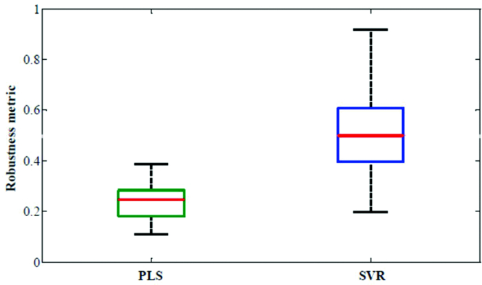
Comparison of wavelength selection for PLS and SVR calibration models in human subjects.

Current FDA recommendations (ISO 15197 guideline) stipulates that for clinical usage 95% of the sensor predictions should be within 15 mg/dL (0.83 mM) of reference for glucose <75 mg/dL (4.2 mM) and within 20% for glucose ≥75 mg/dL (4.2 mM).⁵¹ The percentage of data points satisfying the FDA criteria for our four calibration models are also tabulated in Table 3. While none of the models completely satisfy the 95% criterion (even though the SVR model for 900 spectral points is very close), one can reasonably expect that the deviations from the aforementioned criterion can be overcome by correcting for variations in tissue turbidity and autofluorescence as well as by addressing the physiological lag between blood and interstitial fluid glucose.¹⁶ We expect that our current clinical studies, in collaboration with the MIT Clinical Research Center, encompassing nearly 100 normal and diabetic volunteers will provide the necessary datasets where we can validate our algorithms, including the application of wavelength selected support vector machines. Through these studies, we anticipate the demonstration of clinical feasibility of Raman spectroscopy for noninvasive blood glucose sensing.

Importantly, our results reflect that the selected wavelength subsets are transferable from one human subject to another. To quantify the transferability, we compare the degree of overlap between the wavelength subsets giving the minimum residue error for each of the human subjects. Evidently, if the degree of overlap between wavelength subsets from two human subjects is high, prospective application of the selected wavelength subset from one subject to the other will also provide accurate results. Here, we define robustness metric as the ratio of overlapping spectral points (between selected wavelength subsets of any two volunteers) to the total number of selected spectral points (300). Figure 4 provides box-plots of the robustness metrics for PLS and SVR calibration. The box-plots are generated from the robustness metrics evaluated for all possible combinations in the human subject dataset (i.e., total of 78 data-points from 13 subjects). Clearly, SVR provides a marked improvement with respect to transferability of the selected wavelength subsets. This information can also be readily visualized by a frequency plot showing the cumulative number of times a given spectral point is selected between the different models developed on individual human subjects. Figure 5 provides this alternate representation in which we observe the evident benefits of employing SVR in relation to PLS. The consistency of region selection in SVR is highlighted by the presence of greater structure (higher retention frequency of specific informative wavelengths) as compared to PLS modeling. Taken together, Figs. 4 and 5 illustrates the substantial enhancement of robustness provided by SVR modeling. This enhancement opens new avenues toward construction of universal calibration models based on a small set of features, which also enables the development of Raman instruments employing a smaller set of wavelength sampling channels. A similar idea has been previously proposed by Buydens and coworkers,⁴⁶ arising from their observation of the robustness of SVR with respect to nonlinear effects in NIR absorption and Raman spectra, in regard to the usage of cheaper low-resolution spectroscopic systems for industrial applications. Our results here validate this line of thought in turbid biological media, where multiple interferents (i.e., other Raman scatterers, absorbers and fluorophores) exist.^{48, 52}

Fig. 4

Boxplot showing robustness metric of 300 spectral points for PLS and SVR calibration models.

Finally, we note the implications of these results for the prospects of a miniaturized Raman instrument that can provide adequate detection sensitivity. As is well-known, a major drawback in translation of Raman spectroscopy is the large spatial footprint of the conventional Raman spectrometers, which are ill-suited to meet the needs of a clinical setting. Specifically, continuous glucose monitoring necessitates the development of a hand-held or a wearable device due to the frequency of measurements required for diabetic patients. To this end, Vo-Dinh and coworkers have explored, in a series of publications, the possibility of employing tunable detection filter-based (e.g., acousto-optic tunable filter) serial scanning Raman systems to significantly overcome the footprint drawbacks.^{19, 20} However, since the proposed systems employ serial acquisition of the photons at different wavelengths, a significant number of the Raman photons are not utilized in constructing the final spectrum and consequently larger acquisition times are needed to collect high quality Raman spectrum. While this problem cannot be completely eliminated, appropriate application of wavelength selection can greatly alleviate the problems associated with serial acquisition. For the specific problem of transcutaneous glucose detection, we have demonstrated above that a set of 300 spectral points can provide equivalent levels of accuracy as the full spectrum (900 spectral points). This implies that instead of having to perform serial acquisition over 900 spectral points, one can acquire the Raman photons at one-third of the spectrum, which in turn means the total acquisition time can be reduced by a factor of three. Conversely (and more importantly for glucose detection), one can acquire for longer periods of time (three-fold) at the appropriate wavelengths that leads to more efficient utilization of the important Raman photons. Considering shot-noise limited detection, a three-fold increase in acquisition time translates to a 1.73 times increase in analyte SNR. Using the minimum detectible concentration formulation,^{53, 54} this increase in SNR results in a corresponding reduction in the prediction uncertainty (or rise in precision) by nearly 43%.