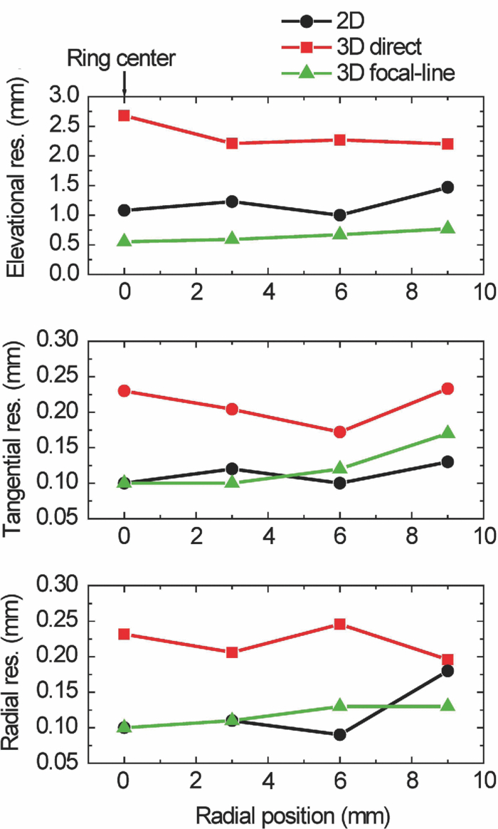
Photoacoustic tomography (PAT) has recently emerged as an important tool for biomedical imaging.¹ By combining optical absorption contrast and ultrasonic imaging resolution, this hybrid technology provides high-resolution images beyond the diffusion limit of penetration depth in conventional optical microscopy technologies.¹ Recently, a full-ring array-based PAT system was developed for real-time functional mouse brain imaging.^{2, 3} The ultrasonic system is cylindrically focused in the elevational direction, and has 512 ultrasonic transducer elements and 64 data acquisition (DAQ) channels with eightfold multiplexing. A two-dimensional (2D) mouse brain cortex vessel image can be acquired in 1.6 s. In the standard reconstruction algorithm,⁴ each element is treated as a point detector. This assumption is valid for 2D reconstruction of an in-plane image, since each ultrasonic transducer element has an in-plane width of 0.3 mm (∼one acoustic wavelength). For this system, however, the standard reconstruction algorithm cannot directly be extended to three-dimensional (3D) space, because the element height (10 mm) and the elevational focus need to be considered. In this letter, we present a novel 3D reconstruction algorithm by treating the focal line of the transducer as an auxiliary line for applying appropriate delays.

1 shows the 3D spatial response of a single ultrasonic transducer element in our array system. Each point in the spatial response map is the maximum amplitude of the spatial-temporal response obtained from the Field II^{5, 6} simulation. Without loss of generality, we used the delta function as the ultrasonic transducer's mechanical-electrical impulse response.

A focal line that goes across the center of the transducer arc (Fig. 1, point O) can be clearly identified in the video. The photoacoustic (PA) wavefront generated from a point in this focal line reaches the entire transducer surface at the same time, maximizing the sensitivity of the receiving aperture. The amount of time delay depends on the position of the point in the focal line. Therefore, we can use this focal line (Fig. 1) as an auxiliary line for applying appropriate delays in the 3D image reconstruction. As shown in Fig. 1, to compute the delay of a point A in the 3D space, we first project A to the x-y plane (B). Point B is then connected to the center point of the transducer (C), crossing the focal line at point D. We then connect A and D, and extend the line to reach the transducer at E. The line AE is always perpendicular to the transducer surface (CD=DE), and is used for calculating the delay time between the imaging point A and the transducer. In the 3D image reconstruction, the original time-domain PA signals from each transducer are back-projected into the 3D imaging space based on the calculated delay times, and are then summed to form the reconstructed image.⁴ The transducer also has a solid acceptance angle determined by the transducer aperture (1). Only PA waves generated within this solid angle can be detected.

Fig. 1

Schematic of the 2D reconstruction, 3D direct reconstruction, and 3D focal-line reconstruction concepts. A: point of reconstruction. A^′: point A projected in 2D reconstruction. A^′C: 2D reconstruction delay. AC: 3D direct reconstruction delay. AE: 3D focal-line reconstruction delay. x-y: 2D reconstruction plane. The focal line is perpendicular to the transducer plane (x-z). (1, QuickTime, 1.7 MB).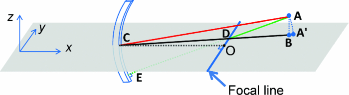

To test the reconstruction algorithm, we first used Field II numerical simulations.^{5, 6} Four PA point sources were evenly distributed along the radial direction over a distance of 9 mm. This arrangement covers a circular area of 9 mm radius in the x-y plane, which represents our typical imaging area. The ring-array was simulated by rotating a single elevationally focused element around the ring center. A 3D dataset was acquired with elevational scanning. This procedure is equivalent to our experimental configuration, where the ring-array is fixed and the sample is scanned along the elevational direction. The transducer parameters are the same as those in the experimental system, i.e., the central frequency is 5 MHz (80% bandwidth), the ring radius is 25 mm, the elevational height is 10 mm, and the elevational focus for each element is at 19.8 mm. The mechanical–electrical impulse response, together with the spectral profile of the ultrasonic transducer element, can be found in our previous paper.⁷ We compared the 3D focal-line reconstruction with two other back-projection algorithms: 2D reconstruction and 3D direct (without the use of the focal line) reconstruction. In the 2D reconstruction, in-plane images are reconstructed individually in 2D space, and then the reconstructed images are stacked together to form a 3D image. Since the 2D reconstruction assumes that all signals are generated within the 2D reconstruction plane (x-y), signal generated from an out-of-plane object (A) is falsely projected to a point A^′ (Fig. 1) in the reconstruction plane with the same time delay (A^′C = AE). Therefore, out-of-plane PA sources always appear as artifacts in the 2D reconstructed image. In the 3D direct reconstruction, all the elements are treated as point detectors, and the time delay to the center of the transducer is employed for back-projection. For a fair comparison between the 3D direct and the 3D focal-line reconstructions, the same solid acceptance angle is applied in both methods. The distances for the time delays employed for the three reconstruction algorithms are shown in Fig. 1.

Figure 2 shows the resolution analysis along the radial, tangential, and elevational directions. The resolutions are defined as the full-width-at-half-maximum (FWHM) of the reconstructed signals in the corresponding directions. It can be seen that when the point sources are located within the reconstruction plane, the 2D reconstruction provides satisfactory radial and tangential resolutions. However, when the point sources are out of the reconstruction plane, 2D reconstruction generates artifacts and renders poor elevational resolution, because it assumes all signals are generated within the 2D reconstruction plane (Fig. 1). The 3D direct reconstruction renders the poorest resolution in all directions, because it does not consider the element aperture in the elevational direction and thus employs incorrect delays. Compared to the 2D reconstruction, the 3D focal-line reconstruction provides comparable in-plane resolution, and improves the elevational resolution by 40%. Moreover, the focal-line method provides a uniform resolution in a larger field of view.⁸

Fig. 2

Comparison of image resolutions of different reconstruction algorithms.

In addition to improving the image quality, the 3D reconstruction method also accelerates 3D scanning. To acquire data from all 512 elements, 64 DAQ channels are multiplexed 8 times, which takes 1.6 s. In the conventional stepwise scan, the sample must remain still at each elevational location for 1.6 s, before moving to the next height. With the 3D reconstruction, continuous scanning can be accomplished, where each group of 64 channels acquires signals at different heights. With an appropriate scanning speed, continuous scanning can record the same amount of data as in the stepwise scan, while saving the stepwise transition time.

To experimentally validate the proposed technique, we imaged a human hair embedded in a gelatin phantom. The scanning speed of the motor was set at 0.1 mm per 1.6 s. The illumination source was an optical parametric oscillator laser, and the laser light was homogenized by a light diffuser. Figure 3 shows the 2D and 3D focal-line reconstructed images. For a better illustration, the same threshold and color scale have been applied on both images to enhance the contrast of the hair. By averaging the elevational (z-direction) FWHM along the hair, we found 3D reconstruction improved the elevational resolution by 30% (1.05 mm versus 1.34 mm), which is not as great as in the simulated data, mainly due to noise fluctuation and small variations in the individual elements’ focusing. The signal-to-noise ratio (SNR) was evaluated by using the ratio of the hair signal to the standard deviation of the background. We found that the 3D focal-line reconstruction improved the SNR by two times. This is because the 3D reconstruction utilized all signals generated within the 3D acceptance angle.

Fig. 3

Reconstructed images of a human hair using (a) the 2D reconstruction and (b) the 3D focal-line reconstruction. z is the elevational direction.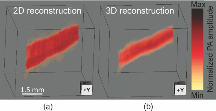

The efficacy of the proposed technique was also evaluated by ex vivo mouse embryo experiments. Mouse embryo imaging has been of particular interest due to its relation to human embryonic studies. Because of the strong light scattering, purely optical imaging techniques normally cannot image embryos older than 12 gestation days.^{1, 9} In this study, we imaged an E15.5 (gestation day 15.5) C57BL/6 mouse embryo (courtesy of Professor Richtsmeier, Pennsylvania State University). The embryo was immersed in a warm 1% Intralipid^™ suspension to induce optical scattering and ensure a more homogeneous incident light distribution. Since blood serves as the main endogenous contrast for PA imaging, we chose two wavelengths (532 and 630 nm) with different molar absorption coefficients of hemoglobin.

Figure 4 shows the 2D and 3D focal-line reconstructed images of the mouse embryo at 532 nm light illumination. Due to the strong blood absorption at this wavelength, major vasculature across the whole body is clearly visible. The spinal cord and ribs also show contrasts, from the microvasculature around the bones.¹⁰ At deeper imaging depths, the heart and liver can also be seen [Fig. 4e]. These two organs are of high interest in the study of early embryonic lethality. Because of the improved elevational resolution, the same image feature dilutes faster in the 3D reconstructed image than in the 2D reconstructed image. For instance, the facial vessel and the tail (arrows) can be seen in all 2D reconstructed images [Figs. 4a, 4b, 4c], while they are only shown in one 3D reconstructed image [facial vessel, Fig. 4d; tail, Fig. 4e]. Another important advantage of 3D reconstruction is the removal of the out-of-focus artifacts. As can be seen from Fig. 4c, when a blood vessel is out of the elevational focus, 2D reconstruction splits the vessel (arrows). In contrast, 3D focal-line reconstruction provides cleaner images over a large scanning depth. 2 shows the 2D and 3D reconstructed images over the whole scanning depth (9 mm) at 532 and 630 nm light illuminations. Because the 630 nm light is less absorbed by blood, internal organs are imaged more clearly.

Fig. 4

In-plane PA images of a mouse embryo at sagittal sections of various depths (2, QuickTime, 1.9 MB): 2.7 mm [(a), (d)], 4.8 mm [(b), (e)], and 6.7 mm [(c), (f)]. Top row: 2D reconstruction. Bottom row: 3D focal-line reconstruction.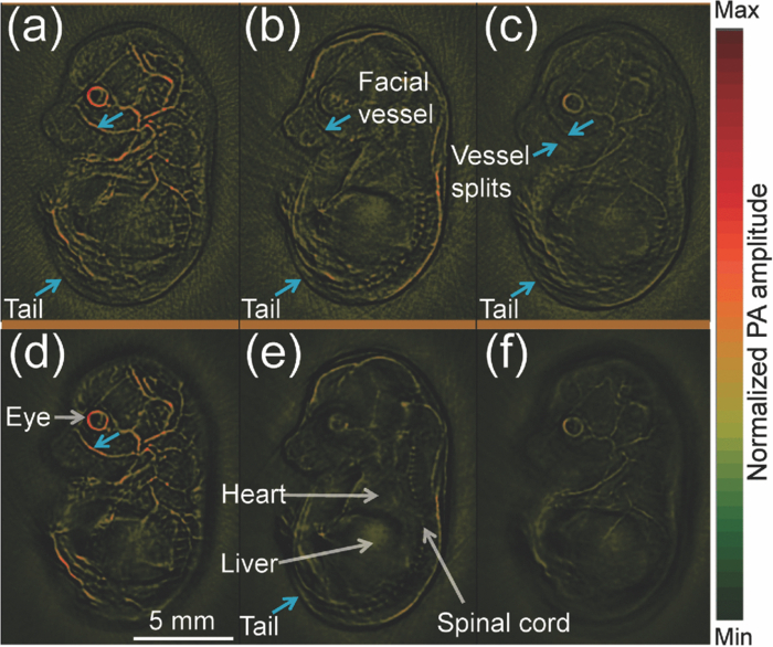

In summary, the 3D focal-line reconstruction improves the elevational resolution of the concave transducer array, and removes the out-of-focus artifacts in 2D reconstruction. Combined with the multiplexed data acquisition system, it also improves the 3D scanning speed without sacrificing the SNR. The technique was successfully applied to image an E15.5 mouse embryo, where whole body vasculatures and internal organs were clearly imaged.