1.

Introduction

It is well documented^{1, 2} that, for people between 18 and 45 years old, civilian and military, internal hemorrhage is the most common preventable cause of death. Early detection of hemorrhage is essential to give medical staff an opportunity to intervene, but when there are no external signs of trauma, autonomic compensatory changes make internal bleeding very difficult to detect.³ Undetected internal blood loss can be manifested by compartment-scale fluid shifts, surface fluid redistribution, and change in blood composition as the body compensates for blood volume loss. The blood hematocrit (Hct) and other physiological measures change, and depending on the measurement site and primary hemorrhage site, some change earlier. Thus, the earliest indicators of hemorrhage are well known but, apparently, we have insufficient means to obtain a continuous real-time record of temporal changes and reactions to external probing. Toward this end, we seek a new means of noninvasively obtaining a continuous time record of relative blood Hct.

Monitoring of body fluids is relevant in many medical contexts, and noninvasive hemoglobin monitors^{4, 5} exist based on optical and other means for probing tissue. To our knowledge, all currently existing noninvasive optical approaches to either total hemoglobin or Hct exploit the coupled oxy/deoxy hemoglobin absorption spectra using at least one hemoglobin isosbestic point(s) (e.g., at 569 or 805 nm). Depending on the desired measurement, at least one other wavelength (e.g., 940 nm) is needed to obtain information about either (i) the relative proportions of the oxy and deoxy hemoglobin or (ii) water absorption as a measure of plasma volume and/or a normalizer for scattering effects. Nevertheless, devices such as oximeters⁶ and hemoglobinometers^{4, 5} produce results that are apparently not sufficiently sensitive, precise, or accurate regarding blood changes to give unambiguous indications to clinicians for diagnosis of internal hemorrhage and determining the need for a transfusion.

Although there is clearly a correlation between increased absorption associated with either increasing total hemoglobin or increasing Hct, the physiological implications of changes⁷ in the two quantities are what determines the utility of their measurement to a practitioner. Total hemoglobin relates more to the oxygen-carrying capacity of the blood, whereas Hct relates more to the viscosity of the blood and may therefore present more unambiguous indications of impending circulatory collapse. Being able to monitor relative changes in blood volume and Hct for a single individual has been shown to be useful for body-fluid management in renal therapy. Using an optical method resembling that used transcutaneously, Leopoldt ⁸ have analyzed extracorporeal blood in the ultrafiltration unit to guide dialysis therapy in renal patients. This approach is only “noninvasive” to a dialysis patient, but it does demonstrate that continuous monitoring of relative changes in Hct is a medical device goal well worth pursuing.

Using a truly noninvasive transcutaneous optical approach Jeon ⁹ reported an absolute mean percent error in estimating absolute Hct within ±8.3% (σ ±3.67). Previously, Jeon ¹⁰ presented a total hemoglobin measurement precise to ±8.5% (σ = 1.142 g/dl). Both papers were based on empirical calibrations of Twersky's treatment¹¹ in which it is assumed that the hemoglobin concentration is 35 Hct.Thus, it seems that for practical purposes we can get only one kind of information from this approach. Testing of another truly noninvasive device⁴ containing Twersky's approach but incorporating advanced signal processing to correct for motion and other human factor defects in the raw measurement also has not produced a consistent assessment of efficacy yet. In fact, invasive approaches that give traditionally acceptable data^{12, 13} are also quite variable¹⁴ due mostly to sampling and handling issues.

Although Twersky's algorithm appears to work quite well for extracorporeal blood analysis,^{7, 15} the noninvasive application of that approach would appear to be deficient in accounting for the presence of other tissues in the probed volume. Also, there is a fundamental limit on the achievable signal-to-noise ratio for blood-volume measurements and quantities derived from them. The raw input into Twersky's algorithm in pulse-modulated devices involves the aforementioned wavelengths and a subtraction of a raw photocurrent at one stage of the cardiac pulse (e.g., diastole), from a raw photocurrent at a different stage (e.g., systole). All existing optical approaches for measuring Hct involve detecting small changes in remitted light intensity in the presence of large steady-state levels containing noise exceeding the shot-noise limit.

In pursuit of improved sensitivity and precision, we note that, unlike approaches based on the Twersky algorithm and absorption, fluorescence-based techniques are essentially zero-background measurements that typically permit 100–1000 times smaller detection limits¹⁶ for absolute concentrations and changes in concentration compared to absorption-based techniques. Thus, we might expect to obtain improved sensitivity and precision in Hct monitoring using a fluorescence-based approach compared to an absorption-based approach. Also, because absorption must precede fluorescence, a fluorescence measurement contains essentially the same species-specific spectroscopic information as an absorption measurement albeit modified by the relative quantum yields of the various fluorophores.

Finally, we note that any absorption or scattering approach of which we are aware employs multiple wavelengths in order to produce an Hct measurement. Obviously, this leads to more complexity in device design and construction; also, the issue of path-length differences becomes important in producing an appropriate algorithm. In contrast, recent advances in enabling technologies make it convenient to examine and analyze nearly all remitted light from tissue due to excitation with a single continuous wave (cw) NIR laser. The elastically scattered light (EE) and the inelastically scattered light (IE) are easily measured, separately, when a charge-coupled device (CCD) detector is employed by simply summing a single frame over different ranges of pixels. Note that although the results we present were obtained using CCD detection, it would be feasible to use optical fiber, an optical filter, a low-grade laser, or possibly only a light-emitting diode and two photodiode detectors to access the same information.

To exploit this situation in seeking clinically relevant information from observed EE and IE time records, we note that the EE and IE constitute two independent observables that can be correlated with two independent volume fractions in a three-phase (red blood cells, plasma, and static tissue) system. The question of how to interpret IE in terms of specific materials within the phases cannot be settled in this paper. These materials are not water itself because water has a very weak Raman spectrum and it cannot fluoresce appreciably in the NIR, because the water absorption is negligible. For now, it is sufficient to note that all the phases contain materials that fluoresce under our excitation conditions and, thus, it is reasonable to include a contribution from all the phases to the net fluorescence.

Stated differently, our basic hypothesis is that the time dependence of the optical properties of skin tissue in vivo are mostly determined by the disposition of the blood in the probed volume. With our practical goal in mind, we note that one must measure both plasma volume and hemoglobin volume to obtain the Hct. Both the EE and IE are modulated by “physical” optics effects (i.e., turbidity and absorption) because they determine the propagation and attenuation of both incoming and outgoing light. In addition, IE results from Raman scattering and fluorescence (i.e., spectroscopic or “chemical” optics effects, which involve changes in quantum states). Therefore, it is reasonable to presume that EE and IE represent two independent observations that can be used to obtain the volume fractions of two independent phases; the plasma and the RBCs. Having these two quantities is equivalent to having the Hct and the total blood volume.

In what follows, we first give some details about how to perform the measurements whose results we describe later. We show raw experimental data typical of probing volar side fingertip skin with NIR radiation in order to give an explicit definition of the EE and IE. We then provide a physical basis for our algorithm by presenting a model that is consistent with the anatomy and function of the skin and the geometry of the probing. We present some simple demonstration data to establish that this approach can actually provide a noninvasive way to monitor changes in the Hct and should be investigated further. Our primary goal in this paper is simply to show that it is possible to monitor changes in the Hct by analyzing scattering intensities.

2.

Experimental

The main features of the methods and instrumentation^{17, 18} used to obtain the scattered intensities as well as the results of applying radiation-transfer equation (RTE) modeling to these measurements⁵ are reviewed here. We probe the volar side of human fingertips, as indicated in the schematic diagram in Fig. 1, using 200 mW of continuous-wave 830-nm excitation that impinges on the skin at 53 deg to the normal, through a 2.1-mm aperture in a 0.635-μm-thick sheet of spring steel. Pressed against the spring steel under external control using only the force needed to maintain optical registration with the collection system, the skin (i.e. soft matter) extrudes a small dome <20 μm into the aperture. The RTE model must consider this profile and its effect on the angle of incidence and propagation of the incident and secondary light to obtain qualitatively accurate results. The remitted light is collected at a ∼f2.1, and a Semrock “Razor Edge” filter is used to simultaneously reduce the Rayleigh scattered light and adjust the dynamic range of the EE and IE as indicated in Fig. 2. A careful measurement gave ∼1 μW total power (i.e., IE + EE reaching the input of the spectrograph slits). When integrated, but without inserting the Razor Edge filter, the EE is approximately five to six orders of magnitude greater than the IE. After being dispersed in the spectrograph, the light is detected by a –45°C Critical Link MityCCD-E3011-BI CCD camera (not shown). A single 20-ms frame as used for all the data in this paper is shown in Fig. 2.

Fig. 1

Schematic of apparatus and layout for measuring scattering.

Fig. 2

Intensity versus frequency from a typical 20-ms frame of Andor CCD. The sections used to calculate inelastic scattering intensity IE (≈500 to 1750 cm⁻¹) and elastic scattering intensity EE (–30 to +10 cm⁻¹) are shown. The low shift integration limit for obtaining IE was chosen by reference to the output obtained when the sample is a nonfluorescent metal and requiring that no EE is included in the IE integral.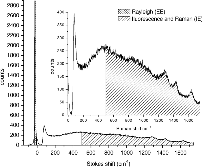

Putting the skin of the volar side of in vivo human fingertips in registration with any optical system must properly deal with human factors. We utilize a position-detection pressure monitor (PDPM) system that detects and records the position of the fingertip skin to within a few millimeters relative to the optical aperture through which all light passes. The position is detected through a series of gold spots surrounding the aperture that also measures the contact area of the finger with the surface around the aperture. The system measures and records the position and contact area of the fingertip, and also the applied force and pressure. Calibration against absolute standards shows that it allows real-time servocontrol of the applied pressure to about ±10 g-force/cm², but the absolute position of 0 g-force/cm² applied pressure can be uncertain to ±35 g-force/cm². The PDPM can be programed to execute a particular pressure modulation in coordination with the CCD cycle during a spectroscopic experiment.

All this is important in these experiments because, as time passes with constant applied pressure (i.e., an isobaric experiment), the blood and other fluids leave the tissue within the stress field and the surface deforms, increasing the contact area. The time record of the pressure provides a plethysmographic record of an experiment and allows us to unambiguously discriminate optical changes due to pulses from those due to spurious motion and other artifacts (e.g., involuntary tremors). In this way, we know that the optical changes we observe are direct monitors of changes in plasma and RBC volumes in the probed region (i.e., blood movement).

For experiments involving tourniquets, we employ a conventional manual blood pressure cuff so that a known blocking pressure can be applied. An Omron automatic blood pressure cuff (Omron HEM-712C, Omron Healthcare, Inc., Bannockburn, Illinois) was employed to measure the blood pressure and pulse rate of the test subjects. Conventional Hct is obtained using fingerstick blood^{12, 13} and a UNICO centrifuge (UNICO PowerSpin BX C884, Dayton, New Jersey) spinning standard 75-mm Drummond microhematocrit (VWR, Radnor, Pennsylvania) tubes at 11,000 RPM for 5 min for each measurement. All of these were then read by the same person for consistency in estimating the buffy coat.

Figure 3 shows sequential 20-ms CCD frames, integrated over Raman shift, to show how the wavelength-shifted remitted light (i.e., the IE) typically varies in time relative to the elastically scattered light (i.e., the EE). Data have been collected and analyzed from four different individuals spanning ages 19–78, male and female, with complexions including Asian, Mediterranean/Arab, Hispanic, and Caucasian. The results presented are representative of one member of the entire set, but the other members exhibit qualitatively similar responses. Test subjects participated after giving informed consent in accordance with our Crouse-Irving Memorial Hospital IRB approved protocol.

Fig. 3

Integrated inelastic scattered light + fluorescence (IE) and integrated elastic scattered light (EE) as a function of time for a single very short and weak mechanical impulse. Starting at time t = 0 s pressure is ≈30 ±10 g-force/cm², immediately followed by increase by 20 g-force/cm² in 0.1 s to ≈50 g-force/cm² followed by active pressure maintenance, i.e., ±10 g-force/cm² in order to maintain the skin in mechanical registration with the optical system. No laser light was present on the skin when it was placed in mechanical registration (i.e., laser was unshuttered at t = 0 s). (a,b) show same data but at different temporal resolution. (b) shows complementary behavior of IE and EE.

We have shown elsewhere¹⁹ that the short-time behavior visible in Fig. 3 of the IE, but not the EE, is dominated by photobleaching of the static tissues. There are various sources of NIR excited fluorescence, including but certainly not limited to various porphyrins, melanin, and advanced glycation end products (e.g., pentosidine). Each source has a unique spatial distribution and set of photobleaching properties, and at this point, we can be certain that there is a contribution to the total fluorescence from at least all these sources. On a longer time scale,²⁰ in all cases steady state is eventually established, and sometimes sinus-cardiac interactions can be seen. These oscillations can only be seen in a relaxed and silent test subject and can be quickly disrupted by requiring the test subject to speak or otherwise disrupt an even breathing pattern. Generally, the elastically scattered light (EE) varies oppositely to the inelastically produced light (IE) during cardiac pulses.

3.

The Model

Much of our approach is dictated by empirical observation and the results of our modeling,¹⁷ using the radiation transfer equation²¹ (RTE), of propagation of NIR in volar side fingertip skin. It is useful to consider the skin as being composed of a static phase and two mobile phases, with no void volume. It does not seem possible to understand the elastically (EE) and inelastically (IE) remitted NIR observed when probing tissue in vivo without adequately accounting for the total blood content and changes in volume fractions due to processes such as plasma skimming and the Faraeus and Faraeus–Lindquist effects.²² This includes what occurs as a part of homeostasis (e.g., the cardiac pulse) and also what may occur due to externally applied stimuli (e.g., cold-induced vasodilation²³) or just the application of the minimum external pressure needed to establish and maintain mechanically stable registration of the tissue to an optical system.⁵

Our model for the structure of skin is consistent with the well-known anatomy and function of skin²⁴ as well as the accuracy and precision of the parameters needed to implement at least semiqualitatively meaningful simulations. In our model, we assume a relatively thin (100 μm), static, bloodless, and nonviable outer layer (a), covering a somewhat thicker (200 μm) relatively blood-rich layer (b) that is bounded from below by dermis, a less blood-rich layer (c) whose depth is essentially infinite. Of course, in reality the thicknesses of all the layers varies across all test subjects, but as defined, there is always a layer a, which contributes to the time-independent component of EE and IE, only because there is no blood in this layer. There certainly always exists a layer above and sufficiently far away from the distal ends of the capillaries to fulfill this assumption. Layer c can be taken as essentially infinitely thick because absorption and scattering preclude collecting much of light scattered from layer c.

Obviously, the papillary interdigitation of the epidermis and dermis presents a topographically undulating interface so layer b is intended only to represent a contiguous volume containing the perfused viable epidermis. We arbitrarily chose²⁵ layer b to be 200 μm thick because we imagine that it includes only the most superficial blood-filled volume of the epidermis. Furthermore, capillary microscopy²⁶ at 830 nm and lower power than we use routinely can image to a depth of roughly 200 μm; thus, it is clear that with this as layer b thickness, we would be correct in assuming a strong signal could be obtained. This image is consistent with the thermoregulation function of blood, which requires a thin blood-rich layer sandwiched between layers with lesser perfusion. In addition, we envision the majority of blood vessels probed are capillarylike so that the RBCs are in single file and layering effects leading to multiple scattering effects cannot occur.

The most superficial tissues²⁴ (i.e., capillaries) will contribute the most to optical effects and have long limbs oriented perpendicular to the skin surface, affording the closest approach between the blood and the external temperature. The arteriovenous shunts and anastomeses responsible for active thermoregulation are somewhat deeper²⁴ and contain less blood under homeostasis at ambient temperatures not too different from 37°C. Given the visual appearance of capillaries in photomicrographs of skin cross sections (i.e., the aspect ratio of the capillaries), capillary lengths should be on the order of 10² μm. This choice is consistent with topographical maps of subsurface structures (i.e., capillary networks produced by laser Doppler velocimtery²⁴ as an easily observable region defined by the presence of RBCs). Choice of a particular value for the thickness of layer b is required for our calculations but given the magnitudes and inherent uncertainties of the optical constants available for use in our model, and the fact that layer b can be expected to change across test subjects, a choice of 200 μm is reasonable for an average “middle” layer thickness that would display the effect of the RBCs on the net optical properties of volar side ridged skin tissue in vivo.

In applying the RTE,¹⁷ we employ the single scattering limit. The physical presence of capillaries is not as important as the mobility they extend to the blood. It is essential that the motion of RBCs and plasma be accounted for separately. The fraction of each layer that is not blood (i.e., not RBCs and plasma) is considered “static” in that it deforms under external pressure but does not move. Note that we do not consider specific cell types in skin (e.g., melanocytes, keratinocytes, etc.). The optical transport coefficients^{27, 28} (μ_s and μ_a averaged over cell types) of normal dermis and epidermis are not very different from each other. Different cell types may have significantly different fluorescence and Raman contributions but with respect to attenuation of the NIR light by elastic scattering and absorption, they are quite similar.

The optical constants are measured in vitro and as noted by the authors,²³ there is wide variation across samples possibly in large part due to sample preparation, which may quite possibly lead to systematical differences from the in vivo values. These comments apply specifically to low spatial resolution (≈10² μm) probing without the spatial resolution afforded by microscopy or confocal methods for which greater detail may be justified. Simple assumptions about cell sizes suggest that we probe 10⁵–10⁶ cells and their corresponding perfusion and extracellular spaces and contents.

The need to account for the effect of variation in blood content when probing tissue with NIR light becomes clear when one considers the composition of each layer (shown in Table 1) and the literature optical coefficients of plasma, RBCs, and static tissue (shown in Table 2). Although static tissue has, by far, the largest volume fraction in the probed tissue, so that the vast majority of collected EE and IE originates from processes in static tissue, the RBC scattering coefficient is much larger than that of plasma or static tissue with the result that even small decreases in RBC volume fraction result in large relative increases in collected EE. There are related effects on the remitted Raman scattered light, but that is beyond the scope of this paper. In fact, the contribution of fluorescence to the integrated IE is substantially greater than the contribution of Raman; thus, unless stated otherwise, we consider only the fluorescence component when referring to the IE. IE is produced subsequent to an absorption event, via μ_a, but also reflects the fluorescence quantum yield;²⁹ thus, although the absorption coefficients of static tissue and RBCs are nearly equal at 830 nm and substantially greater than that of plasma, the greater the RBC content is, the greater the observed fluorescence. This is reflected in the assumed values of inelastic scattering (fluorescence) coefficients used in the radiation transfer equation simulations, also shown in Table 2.

Fig. 14

Volume fractions and Hct calculated from the data of Fig. 13. The two free parameters in the algorithm were obtained by minimizing the standard deviation in the Hct over the first 50 s (before application of the tourniquet). Both calculated volume fractions increase gradually when the tourniquet is applied and drop quickly to their initial values when it is released. The Hct follows roughly the same pattern, but shows some residual effects after tourniquet release.

Table 1

Assumed volume fractions of the three phases in the three layers.

Table 2

Absorption and scattering coefficients from literature and assumed inelastic emission coefficients for the three phases.

The Hct is the ratio of the RBC volume fraction to the sum of the RBC and plasma volume fractions, that is, the fraction of the mobile tissue volume that is RBCs. The two volume fractions can be calculated from the two observables, IE and EE. In principle, values for six scattering coefficients—three for elastic scattering and three for inelastic—must be estimated and used in calculations with the RTE model. We show the results of such calculations in Sec. 4. These results suggest an algorithm for calculating Hct from measured IE and EE, also discussed in Sec. 4. In Sec. 7, we present some recent in vivo human clinical results that illustrate the use of this algorithm.

4.

The Algorithm

Our model¹⁷ permits calculation of the intensity of scattered radiation from all three phases that is detected outside the skin, given volume fractions, absorption coefficients, and scattering coefficients for the three phases. We have shown¹⁷ that it accounts for the observed variation in detected intensity with changes in geometric parameters (placement of source and detector, etc.) and volume fractions. Calculations using our model will now be used to obtain relations between the coefficients that enter our algorithm and to see the form of the functionality connecting the phase fractions and the observed EE and IE. Of course, the values of the parameters differ between individuals; thus, we do not place great emphasis on their exact values. The important point is that the relations we derive are not strongly affected by variation in these parameters.

On the basis of our earlier experiences^{17, 18, 19, 20, 22} with a range of skin types and a specific experimental apparatus, we use geometric parameters as follows for the RTE calculations.¹⁷ The dome formed when the fingertip is brought into registration with the 2.1-mm-diam optical aperture is assumed to be a spherical cap with radius 0.1 cm and height 0.005 cm. The origin of coordinates is in the center, 0.005 cm below the top of the dome. The angle between the direction of the incoming beam and the vertical is 0.980 rad, and the origin of the beam is chosen so that the center of the beam crosses the skin surface at the top of the dome (actually at x = −0.0025404 cm, y = 0.004997 cm). The detector center is at x = 0.015 cm, y = 0.013 cm. The dome height is estimated from experiment.

The values of the parameters characterizing the skin for the simulations are given in Tables 1, 2. The volume fractions in Table 1 are based on estimates^{30, 31} of the average capillary density, capillary dimensions and an Hct of 0.10 for the blood in the most vascularized second layer. Consistent with general anatomy, layer c was given 10% of the total blood fraction of layer b, which extends from the top of the capillary loops down to but not including the superficial dermal plexus. The calculations show that, for all three phases, the contribution of layer c is much less than that of layers a and b, so that the assumptions made for layer c are not critical. Furthermore, even if the total blood fraction is assumed to be as high as 0.05, consistent with Jacques’ estimates³² for well-perfused skin, such as fingertips, the scattering length is very long compared to the dimensions of the layers and the single scattering limit is appropriate. The estimates in Table 1 are more appropriate to forearm skin, but in any case, we are in the single scattering limit and our RTE approach is justified.

The volume fractions (see Table 1) sum to unity, implying that there are no voids. This is summarized in Eqs. 1, 2 using ϕ for each of the volume fractions (i.e., RBCs, plasma, and static tissue in each layer),

In our model, the absorption and inelastic scattering coefficients, weighted by phase-volume fractions, are added to give the attenuation coefficient for each layer. The calculated elastic scattering intensity from each point is proportional to the corresponding elastic scattering coefficient, and the inelastic scattering intensity is proportional to the inelastic scattering coefficient. Both are proportional to the (attenuated) NIR intensity at that point.

Because the actual collected intensities depend on the size of the collection circle and the range of wavelengths accepted by the collection optics, only relative values are significant. Good agreement between theory and experiment, relative to changes in geometrical parameters, was obtained¹⁷ by summing the contributions from each phase and each layer. Obviously, one can “measure” only the total elastic and inelastic scattering, but one can “calculate” the separate contributions, as shown in Figs. 4 and 5. It is clear that the contribution of layer c is unimportant because of the increased path length and attenuation. Thus, because there is essentially no blood in the stratum corneum and the nonviable epidermis, it is the blood-volume fractions in layer b that are measured, and the Hct depends mostly on volume fractions in layer b,

Fig. 4

Using the RTE model of Ref. 17, we calculated elastic and inelastic scattering intensities from (a) static tissue,(b) red blood cells, and (c) plasma plotted versus volume fraction of RBCs. Squares designate outermost layer, circles are from the middle layer, and triangles are from the innermost layer. Total blood-volume fraction is assumed constant; average volume fractions of RBCs and plasma are 0.004 and 0.036, but the Hct is varied. The fits to these data lead directly to the coefficients in Eqs. 8, 9.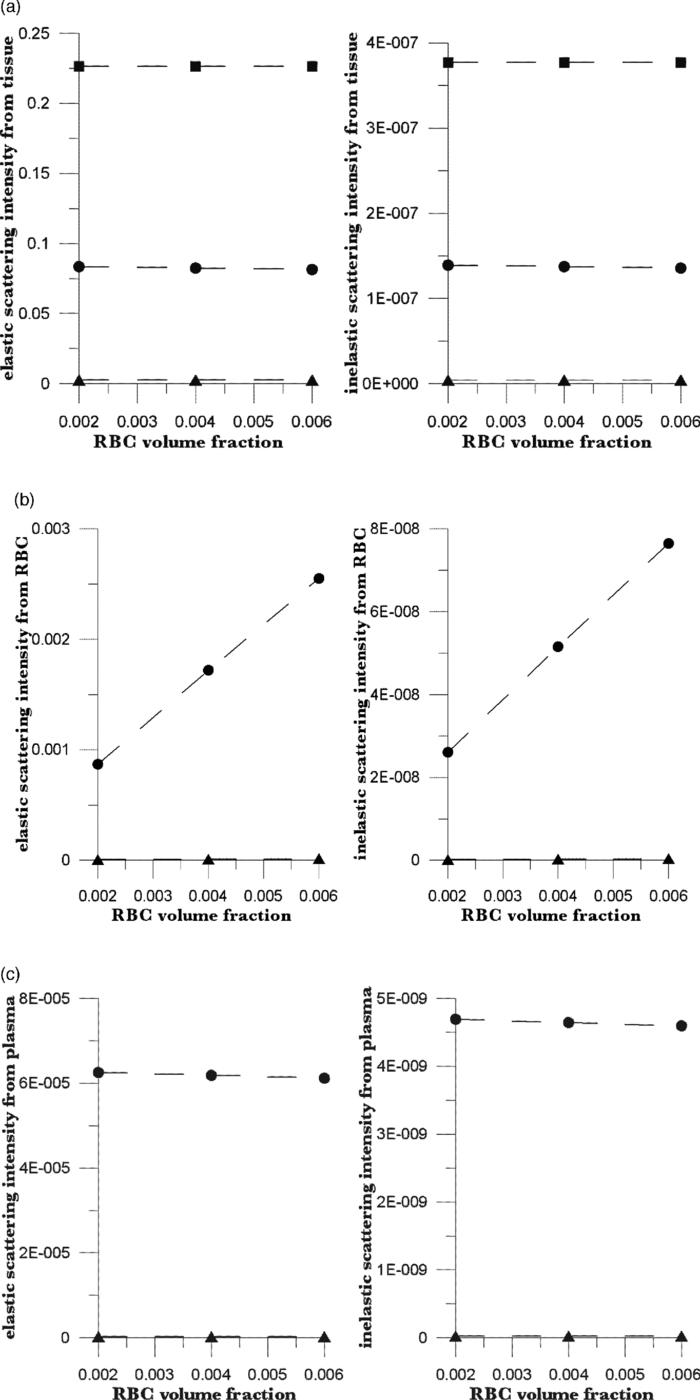

Fig. 5

Elastic and inelastic scattering from (a) static tissue, (b) red blood cells, and (c) plasma plotted against volume fraction of plasma. Squares are from the outermost layer, circles are from the middle layer, and triangles are from the innermost layer. Total blood-volume fraction is constant; average volume fractions of RBCs and plasma are 0.004 and 0.036, but the Hct is varied as indicated. The fits to these data lead directly to the coefficients in Eqs. 8, 9.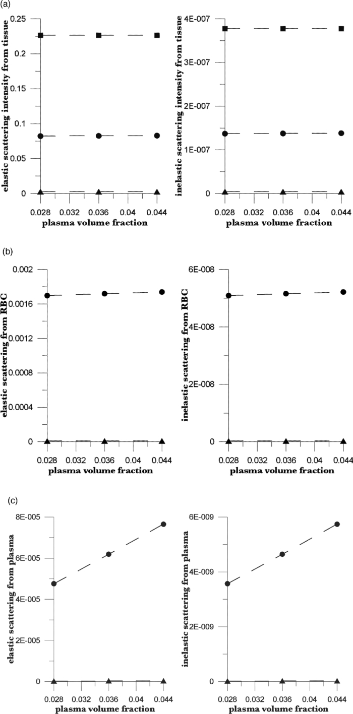

More importantly, the results of these and many other calculations show that the elastic and inelastic scattering intensities are linear functions of the volume fractions of the three phases in layer b (r ² > 0.999 for the data shown). The linear dependence is both direct (the amount of scattering from any phase at any point is proportional to the volume fraction of that phase at that point) and indirect (the scattering is proportional to the incident light intensity, which is determined by the attenuation, and the attenuation of the scattered light before reaching the detector is linear in the volume fractions). It is important to note that the observed values of EE and IE depend on how they are measured and on the geometrical parameters of the system, such as the probed volume, the frequency range considered, and the incident laser flux.

Using Eq. 1, we may write the linear dependence as

We can conceive of at least two ways to determine values for the parameters ϑ_j. We can (i) attempt to calculate the parameters via a series of numerical RTE calculations or (ii) determine the parameters empirically based on measurements of EE and IE variation in response to independently known physiological stimuli.

5.

Numerical Calibration

Using our model¹⁷ with the parameters of Table 1, and values of ϕ_r and ϕ_p centered around 0.004 and 0.036, respectively, we calculated the EE and IE for systematically chosen values of blood volumes as shown in Figs. 4, 5. Each graph gives the results of calculations for which the total blood volume (i.e., the sum of the RBC and plasma volumes) is held constant, but the Hct is varied. The best bilinear fits to the summed contributions from all three layers were (C indicates calculated quantities):

Because EE is proportional to EEC and IE is proportional to IEC, we can write

This leaves only two normalizing parameters to be determined. Because our RTE calculations assume ϕ_r = 0.0040 and ϕ_p = 0.0360, ϑ₁ = EE₀/1.003815, and ϑ₄ = IE₀/1.000814, where EE₀ and IE₀ are to be measured at some reference point, such as a particular applied pressure relative to the diastolic and systolic blood pressures, or a particular temporal position relative to the cardiac pulse, at which the assumed volume fractions actually obtain.

Solving Eqs. 6, 7 for the volume fractions gives

The Hct is then given by Eq. 3. Note that, if IE = IE₀ and EE = EE₀, these equations yield ϕ_r = 0.0040, ϕ_p = 0.0360. Equations 8, 9 show how the two volume fractions ϕ_r and ϕ_p, which give the Hct, may be calculated from measured IE, EE, EE₀, and IE₀ quantities.

There are a number of ways to utilize this algorithm. We first give a very brief example, using the data of Fig. 3, smoothed by taking 50-point averages. The values of ϑ_j are obtained from EEC and IEC as given above. The values for EE and IE are 75208 and 83205 counts at 66.5 s, 75511 and 82521 counts at 66.9 s, and 75438 and 82877 counts at 67.3 s. Using Eqs. 8, 9 with the first point corresponding to EE₀ and IE₀, the second point gives ϕ_r = 0.00765 and ϕ_p = 0.07276, and the third point gives ϕ_r = 0.00692 and ϕ_p = 0.06426. The Hct values for the latter two are 0.0951 and 0.0972, showing an apparent decrease from the value assumed for the first point, 0.10.

Because of the way the equations are cast and the parameters are determined (i.e., EE0 and IE0 are obtained from the test subject being monitored), the average Hct returned will be the assumed value regardless of test subject and the real Hct. Also, a change by a certain amount in actual in vivo Hct for one test subject can be expected to produce a different change in IE and EE for a different test subject. This will constitute the calibration challenge for this approach, suggesting that we explore its application when external means are used to vary Hct and blood volumes.

Because our goal is to monitor plasma volume, RBC volume, and Hct changes continuously and in real time, we show how to implement the algorithm, considering data with a realistic systematic defect (e.g. photobleaching).⁶ Figure 6 shows the result of analyzing a segment of the measured EE and IE of Fig. 3 using Eqs. 8, 9. The data were first subjected to 11-point average smoothing. To reduce the effect of the photobleaching on our calculations, IE₀ and EE₀ were obtained by averaging IE and EE over the 200 points for 50 ≤ t ≤ 60 s. Then, EE/EE₀ and IE/IE₀ were calculated for all points for t ≥ 60 s. Note that, in principle, EE₀ and IE₀ are functions of the homeostatic state (i.e., blood pressure, heart rate, metabolic state) of the physical specimen so that, for a given apparatus and specimen, a single set of EE₀ and IE₀ values should suffice. Because tissue emits well-known “autofluorescence” that bleaches in time, one should be sure that steady state with respect to this process has been achieved before calculation of EE and IE in order to show effects of blood movement.

Fig. 6

Calculated volume fractions for RBCs, plasma, and Hct, derived from data in Fig. 3 using Eqs. 8, 9. The reference IE₀ and EE₀ levels were averages from 50 to 60 s, as described in the text. (a) shows all results and (b) shows the section from 60 to 75 s.

If we use the parameters derived from the attenuation coefficients and volume fractions used for our original RTE model¹⁷ (appropriate for forearm skin), calculated volume fractions have negative values and/or are unrealistically large, as shown in Fig. 6. Although the values of the parameters that enter the RTE simulation are uncertain, they cannot be chosen arbitrarily if the algorithm is to produce reasonable volume fractions. Thus, using parameters derived directly from an RTE calculation without any optimization of anatomic parameters, the blood-volume fractions sometimes take negative values so that the volume fraction of skin is >1. However, the calculated Hct is affected only when one or both volume fractions are close to zero.

6.

Empirical Calibration

We now show how to parametrize the algorithm using experimental results. For this purpose, Eqs. 8, 9 can be written as follows:

Additional constraints can be obtained from changes in EE and IE that can be correlated with known physiology. From Eqs. 10, 11, we find

We note that normally with each cardiac pulse³³ about 75 ml of 0.45 Hct blood is injected into the arterial side of the 4000-ml total supply. Uniformly distributed, this would result in a 1.9% transient increase in blood volume (i.e., in both ϕ_r and ϕ_p assuming constant Hct). Thus, we can assume that with each pulse ϕ _r and ϕ _p increase by 0.000076 and 0.000684, respectively. The raw data in Fig. 3 shows a −2.08% and +2.63% change in EE and IE, respectively, with each cardiac pulse (i.e., systolic EE and IE minus diastolic EE and IE). These two conditions can be inserted into Eqs. 12, 13 to generate two more constraints on the values of the parameters a–f,

These equations constitute two additional constraints,

Figure 7 shows another empirical observation that leads to two constraints on the parameters. A test subject fingertip was tissue modulated between 60 and 276 g-force/cm², and as shown, EE increased by 3.03% and IE decreased by 9.6%. In obtaining these results, the maximum applied pressure was three to four times the normal systolic blood pressure; thus, the amount of blood displaced is three to four times the amount displaced by a pulse. We estimate the changes in ϕ_r and ϕ_p based on (i) the applicability of the Poiseville–Hagen equation to optimization in the cardiovascular system³⁴ and (ii) the variation in appearance of tissue-modulated spectra with varying amounts of modulating pressure.⁸ Although we probe the capillaries, they are fed by the superficial dermal plexus, with vessels large enough to demonstrate well-known microcirculation anomalies⁹ (i.e., plasma skimming and the Faraeus and Faraeus–Lindquist effects), associated with nonproportional plasma and RBC movement. Under greater applied pressure, relatively more plasma is expected to move than RBCs because the viscosity of plasma is less than that of RBCs. Under our experimental conditions, we estimate the discharge Hct as 0.075. The decrease in ϕ_r is therefore 3×0.019×0.004 = 0.000228 and the decrease in ϕ_p is 4×0.019×0.036 = 0.002736. This corresponds to three and four times the amount of RBCs and plasma moved by a single pulse. Putting the decrease in ϕ_r from its reference value equal to 0.00024, Eq. 12 gives

Fig. 7

IE and EE as functions of time for two different modulation cycles. In one cycle, the pressure went from low = 60 g-force/cm² to high = 200 g-force/cm², and in the other, the opposite is true. (a) EE for low to high, (b) EE for high to low, (c) IE for low to high, and (d) IE for high to low. Trials (a) and (c) were used to provide the calibration in the text.

Similarly, Eq. 13 gives

Thus, there are various approaches involving empirical observation of IE and EE modulation, associated with known physiological effects, to obtaining constraints on the six parameters.

The above examples yield four constraints on the six parameters. We determine the remaining two parameters by minimizing the standard deviation of the Hct from the mean over some time range of measurement. This is justified because, normally, Hct is constant under homeostasis.³⁴ The mean value will be ∼0.1 because the reference values of ϕ_r and ϕ_p are 0.004 and 0.036, respectively. Again, we emphasize that the assumed values are not important—what matters is the deviation of the calculated ϕ_r and ϕ_p from the reference values.

We now apply the above equations to the data of Fig. 3, analyzed in Fig. 6. The values of EE₀ and IE₀ were obtained, as before, from the data for 50 sec ≤ t ≤ 60 sec; the physiological constraints discussed above were used to reduce the number of parameters in Eqs. 10, 11 to two, and the remaining two parameters were determined by minimizing the standard deviation in the Hct over the same time interval. Then, the six determined parameters were used in Eqs. 10, 11 to calculate the volume fractions ϕ_r and ϕ_p for all t ≥ 50 sec. The results are shown in Fig. 8.

Fig. 8

Results of analysis of data of Fig. 3. Data from 40 ≤ t ≤ 50 s was used to establish EE₀ and IE₀, and the two free parameters in the algorithm were determined to minimize the standard deviation of the calculated Hct. The parametrized algorithm was applied to all data for 50 ≤ t ≤ 100 s, giving the results shown. (a) calculated volume fractions and (b) calculated Hct.

It is immediately apparent that this method of parametrization leads to much more stable results than the previous one. Volume fractions vary only in a relatively small range and never go negative. The variation in the Hct is extremely small, less than two parts in a thousand over the entire range: note that the parameters were chosen to minimize the standard deviation of the Hct for the first 10 seconds of data. The results of this analysis indicate that the Hct, like the two individual volume fractions, gradually increases over the measurement time.

7.

Results

The choice of what to use for the values of EE₀ and IE₀ is critical in applying this algorithm to real data, and thus for this paper, we analyze data from a single test subject because, for practical purposes, we are looking to monitor a single patient with respect to possible internal hemorrhage. We will consider cross-subject variability in a separate paper. We have suggested means for calibration based on our interest in maximizing our chances of observing subtle changes in Hct and/or total blood volume. We choose to (i) determine a set of a–f parameters as described above using the empirical calibration method and all measurements, in this case, on the same individual, (ii) determine the EE₀ and IE₀ from the data for a specific individual, and then determine volume fractions and Hct. The equations in the calibration section require that the algorithm must produce the assumed values of the volume fractions when the patient is at homeostasis (i.e., the EE and IE are near their averages). It will do so for subsequent times if the EE₀ and IE₀ are determined when first placing a person in the apparatus. The magnitude of any subsequently observed changes in the calculated volume fractions for a given set of changes in IE and EE will vary from person to person, but an indication of change may well be much clearer than with other devices because the fluorescence measurement has inherently better signal to noise.

The assumptions for “normal” volume fractions of RBC's and plasma (i.e., the volume fractions corresponding to EE₀ and IE₀) are determining of the average capillary Hct calculated from the data, but conclusions about the behavior of the Hct in response to perturbations should be relatively insensitive to the exact numerical values chosen within the constraint that this analysis should be correct for single scattering limit systems. We check this by a new analysis of the data in Fig. 3. In this and in all subsequent calculations, we make a more realistic assumption for the volume fractions of RBC and plasma: ϕ_r = 0.012, ϕ_p = 0.028; thus, the reference Hct is 0.30. We use the data from 56 to 64 s, with 11-point smoothing, as our standard, chosen to reduce interference with homeostatic blood-volume changes associated, e.g., with small involuntary movements of the tissue with respect to the aperture, that nevertheless penetrate the active servosystem in use in our device. Thus, EE₀ and IE₀ are the averages over this time series.

The top plot in Fig. 9 shows EE/EE₀ and IE/IE₀, giving an idea of how much variation there is in EE and IE, i.e., ≈2%. Note that the EE and IE have magnitudes on the order of 30,000 and 70,000, respectively, that in the shot-noise limit correspond to raw signal to noise of 175:1 and >250:1 respectively. The raw signal levels are essentially shot-noise limited and, thus, this corresponds to a noise floor in the range of 0.4%, easily attained because the CCD detector has effectively no dark current for the CCD temperature and frame time. The two free parameters in Eqs. 10, 11 were then obtained, as described above, by minimizing the standard deviation of the Hct over the time interval.

Fig. 9

(a) EE/EE₀ and IE/IE₀ for the 8-s time interval (400 points) between 56 and 64 s, using data of Fig. 3, with EE₀ and IE₀ equal to the average values of IE and EE over the interval. Volume fractions ϕ_r and ϕ_p were assumed to be 0.004 and 0.036. The parameters in the algorithm were determined to minimize the standard deviation in the calculated Hct, with the four constraints as discussed in the text. Phase volume fractions (upper curve = ϕ_r, lower curve = ϕ_c) and Hct calculated using these parameters are shown in (b) two plots.

The resulting parameters were: a = 0.02962, b = −0.01610, c = −0.00152, d = 0.06462, e = –0.03626, and f = –0.00037. Calculated volume fractions for plasma and RBCs are shown in the middle plot of Fig. 9; and the Hct in the bottom plot. The calculated volume fractions vary by a percent or two, whereas the Hct varies by only 0.08%. This is not surprising because the parameters were chosen to minimize the variation in the Hct over this data set.

The parameters a–f determined from this time interval were then used to analyze other later parts of the data of Fig. 3. Thus, the measured intensities for 70 through 90 seconds (1001 time points) were treated by 11-point smoothing and analyzed using these parameters, taking EE₀ and IE₀ as the averages of EE and IE over the 56-64 s time interval. Figure 10a shows that EE increases over the time interval, by ∼2%, while IE decreases by ∼14%. This inverse behavior, seen in the pulses as well, has been explained by the fact that the increases of RBCs increases IE (because the fluorescence per unit volume of RBCs is greater than the volume normalized fluorescence of the other phases) but decreases EE (due to screening). Analysis of the intensities using our algorithm gives the results for ϕ_p and ϕ_r in Fig. 10b. Overall, both decrease slightly with time: the slope of the best linear fit for ϕ_r is (–1.71 ±0.03) × 10⁻⁵ s⁻¹ and the slope of the best fit for ϕ_p is (–4.61 ±0.08) × 10⁻⁵ s⁻¹. Because the ratio of average ϕ_r to average ϕ_p is 3/7 and the ratio of slopes is <0.42, the Hct increases slightly over this time interval: slope (4.93 ±0.07) × 10⁻⁵ s⁻¹. This is the same conclusion as that from our previous analysis in which 0.1 was used as normal Hct. This is shown clearly in Fig. 10c, which also shows that the increase is not uniform. (The nonuniformity is also shown by our previous analysis, but it is more evident in the present one.) The long-period oscillations may be due to cardiac-sinus interactions or to other physiological fluctuations, including variation in oxygenation. This could possibly affect the fluorescence quantum yields for the hemoglobin systems, but in any case, these are physiologically small effects as the test subject is comfortably maintaining homeostasis with no external perturbations.

Fig. 10

Data from Fig. 3 for 64.5 < i < 91.5 s were analyzed using the parameters (a–f) calculated from the 56–64 s data (Fig. 9), and values of EE₀ and IE₀ equal to the average intensities over 64.5–91.5 s. (a) Shows EE/EE₀ (solid curve) and IE/IE₀ (dashed curve); they vary inversely. (b) Shows calculated volume fractions for RBC's (lower curve) and plasma (upper curve); both show an overall decrease with time. (c) Shows the calculated Hct, which increases by 2% over the time interval.

As another example of utilizing the algorithm, we consider an experiment in which the homeostatic blood volumes are intentionally perturbed in a manner that may be comparable to an autonomic response to hemorrhage (e.g., shifts in peripheral body fluids). There are a number of means for accomplishing this;³ here, in analogy to the method used to measure the Hct of a blood sample in vitro, we use centrifugal loading. By “centrifugal loading,” we mean that the test subject rotates the arm about the shoulder with the arm, elbow, and fingertips outstretched so that all joints and long straight members of the circulatory system have a projection along the centrifugal force direction. If the maneuver is properly executed, then the test subject feels tingling in the fingertips after the swinging. Use of conventional centrifuge fingerstick Hct measurements established that the absolute value of the difference between measurements of Hct before and after the centrifugal loading step is roughly three times greater than the variation in Hct readings obtained from consecutive samples going forward in time but without the loading in between. The arm swinging procedure definitely causes blood imbalance in the fingertips, but depending on the timing and execution of the procedure, the time course is apparently variable.

The data from Fig. 3 include measured IE and EE before and after photobleaching equilibrium⁶ has been attained. As noted, to unambiguously and accurately observe and interpret effects of blood-volume changes, it is important to reach photobleaching equilibrium before monitoring EE and IE for quantification. Each set of measurements after executing the arm-swinging protocol was preceded by a mechanical setup process⁵ to establish reproducible placement and applied pressure to the fingertip, followed by a 20-s prebleaching. After this period, IE and EE were monitored continuously for 20 s with a minimum of applied external pressure (i.e., < 60 g-force/cm²). (The data in Fig. 12 were obtained before and just after centrifugal loading.)

Fig. 12

(a) Volume fractions of plasma (upper curve) and RBCs (lower curve) derived from a 20-s measurement of EE and IE (i.e., calibration run before arm swinging). (b) Volume fractions of plasma (upper curve) and RBCs (lower curve) derived from a 20-s measurement of EE and IE after vigorous arm swinging to drive blood into the capillaries. The volume fractions were calculated using the algorithm with parameters derived from the calibration run. (c) Hct as a function of time from the calibration and postswing data sets.

Estimating the rotating arm length as >30 cm and the rotatory motion as 120 rpm, we calculate >4G applied force using the standard relative centrifugal force (RCF) equation.³⁵ For the results that follow, the loading was continuous for a period of at least 30 s. Because G-force induced loss of consciousness³⁶ (GLOC) is known to occur as a result of transient application of two to four G forces to the human body, 30 s of continuous motion 4G force could be expected to lead to transient minor hemoconcentration in the fingertips or leakage through the capillary walls, just as centrifuging leads to hemoconcentration in an Hct tube. Of course, standard centrifuging to measure Hct in a Hct tube usually requires 3–5 min at ≈11 × 10³ rpm, but the distances traversed by the RBCs and the resulting cell packing are much larger than are necessary to observe the in vivo loading effect.

Figure 11 shows the EE and IE from two typical sets of measurements—one immediately preceding arm swinging (a) and the other immediately after 30 s of arm swinging (b). These data have been subjected to 11-point average smoothing. The intensity profiles from the first set were analyzed to obtain the parameters in the algorithm by minimizing the standard deviation in the calculated Hct. These parameters were used to analyze the postswing data, with EE₀ and IE₀ being the averages over the postswing intensities. The results are shown in Fig. 12.

Fig. 11

Elastic (EE) and inelastic scattering (IE) was measured (a) before and (b) after arm-swinging for 30 s. After 11-point smoothing, the intensity profiles were as shown.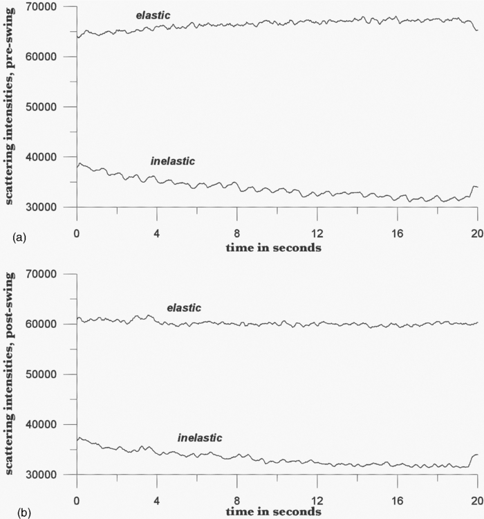

Figure 12a shows the calculated volume fractions of plasma and RBCs for the preswing data. Both decrease slightly with time over the 20-s measurement period. In Fig. 12b, we show the volume fractions of plasma and RBCs for data following swinging, calculated using the parameters derived from the preswing data. Here, the decreases in ϕ_p and ϕ_r with time are much greater; each drops by almost 50%. Figure 12c presents the calculated Hcts before and after swinging. Hct calculated from the preswing data increases somewhat, from ∼0.2911 to ∼0.3094, over the 20-s time period, whereas that from the postswing data decreases from ∼0.3102 to ∼0.2856.

These estimates are from visual examination of the Hcts versus time, but the apparent increase in Hct preswing is an artifact of the fact the 20-s prebleach was not adequate to completely eliminate the decrease in IE with time due to photobleaching. We made this time shorter in order to improve our chance to observe the test subject during the relaxation to conditions of homeostasis and so hemoconcentration dissipated so our measurement cycle could detect it. Nevertheless, the fact that both volume fractions were much higher just after arm swinging shows that the arm swinging indeed pushed more blood into the capillaries of the fingertips. The subsequent decrease of volume fractions with time shows the draining of the excess blood, with the volume fractions returning to their reference values. The fact that the Hct for the postswing data was initially high and decreased over the 20-s measurement period indicates that relatively more red blood cells were pushed into the capillaries by swinging and were trapped there. Because the same cause of the artifact preswing data was also present in the after-swing measurement, if we corrected for this artifact, then the calculated decrease in Hct postswing would be about twice as great.

As a final experiment, we used a manual blood pressure cuff as a tourniquet to induce hemoconcentration. After determining the test subject's blood pressure and pulse rate using an automatic cuff, IE and EE were collected with no applied tourniquet beyond that needed to maintain mechanical registration of the tissue with respect to the optical system, in order to define homeostasis. The applied pressure was maintained by the PDPM at 35 ±10 g-force/cm², the lowest we could maintain (on that day), for 60 s. The tourniquet brought the pressure to its final planned value within five to seven cardiac pulses by a single increase in pressure (in several pumps on the manual bulb), at 60 s. The final pressure was chosen to be just above the systolic pressure in order to insure venous occlusion, which can be confirmed with a stethoscope. Once complete occlusion was established, it was maintained without modification for 60 s. Thus, at 120 s from establishing homeostasis, the tourniquet was released as quickly as possible. The associated changes in EE and IE can be seen in Fig. 13.

Fig. 13

EE/EE₀ and IE/IE₀ versus time for application of tourniquet at t ∼ 60 s and release at t ∼ 120 s. Prebleaching was performed before data collection. Plasma and RBC volume fractions and Hct, derived from this data, are shown in Fig. 14.

Both scattering intensities decrease gradually after the tourniquet is applied and rebound quickly to their original values when the tourniquet is released. The decrease is ∼10% for EE and ∼20% for IE. Data from the first 50 s were used to calculate EE₀ and IE₀. The two free parameters in the algorithm were determined by minimizing the standard deviation in the calculated Hct over the same time period. The resulting RBC and plasma volume fractions, and the Hct, are shown in Fig. 14. Both volume fractions rise gradually during the period over which the tourniquet is applied, showing that the main effect is trapping blood in the irradiated volume. When the tourniquet is released, both volume fractions drop quickly to their pretourniquet values. The Hct, because of our parametrization, is much more constant, changing by only 0.5%, but also increases on application of the tourniquet and decreases on release. The increase, which is a little sharper than the increases in volume fractions, shows that relatively more red blood cells are trapped than plasma. Interestingly, the Hct shows some posttourniquet effects. After release, the Hct drops to its original value, but then increases gradually to a value about 0.5% higher. By 200 s, it has leveled off; our measurements do not go far enough to determine how long it takes to come down again.

For direct comparison, three test subjects exercised the tourniquet maneuver using a blood pressure cuff pumped above systolic pressure for 2 min four times in a week's time span and the conventional Hct determination technique was employed. For each subject, two to four data points were taken both before and after the maneuver each day, which yielded a total number of 61 data points, 30 before and 31 after. The average Hcts before applying tourniquet were 0.3794, 0.3715, and 0.4055; whereas the averages after were 0.4020, 0.3811, and 0.4138, respectively. The statistics show a clear trend of increased Hct after the tourniquet is applied. To support the statement in a more statistically meaningful way, the null hypothesis is tested by splitting the raw 61 data points into two sets, 30 before and 31 during application, without differentiating test subjects and the dates on which the experiments are performed. The result yields a p-value of 0.039, which is significant at >90% confidence to reject the null hypothesis that assumes there is no Hct change due to the tourniquet. Moreover, within any set of personal Hct values, the behavior is much more consistent; thus, the statistic just quoted tends to underestimate the Hct change on a single-person basis. Therefore, we used personal average Hct as a normalizer for each individual, and instead of using raw Hct, the relative change of Hct was used to test the null hypothesis. A p-value of 0.0219 resulted, even more strongly supporting the probability that Hct increases with the tourniquet applied, as shown in Fig. 14.

8.

Discussion

Using a model based on the radiation transfer equations, semiquantitative agreement between calculated and observed spatial and temporal dependence of the IE and EE was readily obtained.¹⁷ Systematic exploration of the parameters used with the model would likely produce much better agreement with experiment. The values obtained for the scattering and absorption coefficients and the fluorescence quantum yields would be reasonable approximations to the parameters in vivo, although we are not aware that these numbers are currently known with any degree of certainty or precision. Given more experience with this analysis, perhaps they could be compared to potentially corresponding parameters^{27, 28, 29} measured in vitro. The calculations also clearly showed that, when the total blood volume was constant, a decrease in the Hct caused an increase in the calculated EE. Thus, if the total blood volume increase during a cardiac-driven pulse was associated with an increase in RBC volume fraction, we should expect the IE to increase and the EE to decrease, as observed. As mentioned earlier, these general statements are supported by observations and calculations in the general range of blood-volume fractions that are attainable without extreme physiological disruptions. Under conditions of much greater or lower total perfusion and Hct, perhaps other results may be possible.

Because we obtained agreement with empirical observation¹⁷ by summing the contributions to the EE and IE across the phases and layers, we were confident that, despite or perhaps because of the geometric specificity of the experiment, the general conclusions were valid. In particular, IE and EE were linear functions of the phase fractions [Eqs. 4, 5]. Thus, the two independent variables ϕ_r and ϕ_p should be calculable from the two measured parameters IE and EE. Six parameters are required for the two linear relationships. We have suggested several approaches to obtaining values for these parameters; we hope in the future to improve these estimates and ultimately obtain an absolute calibration against an in vivo physiological standard. This is certainly one of the strengths of the absorption-based Twersky approach; it achieves agreement to within 8% of absolute Hct measurements.

In this regard, we note that, for normal skin with not particularly dark pigmentation, the effect of variation of skin types on in vivo spectroscopic analysis^{37, 38, 39, 40} is not as great as to preclude observation of effects of variation in perfusion. We suggest that the effect of blood perfusion on the apparent turbidity is greater than the effect of skin-layer thickness and hydration state. Because the perfusion is affected by many things (including the manner of mechanical registration of an aperture, window, or fiber bundle to the surface of the probed skin), experiments should explore the variation of the observed spectra with systematic variation in the mechanical coupling to the skin surface.

Notwithstanding these sources of variation of EE and IE, our immediate practical interest is with respect to a particular person across time. As we have shown, the algorithm is potentially self-calibrating in the first few seconds of optical probing of a specific individual. Also, although waiting until autofluorescence photobleaching has reached steady state before beginning Hct monitoring will produce more accurate and precise results, it appears that a set of parameters can be obtained by empirical calibration before photobleaching has reached steady state, which will still produce reasonable results for later times. In an emergency situation, this might be necessary. We expect decreasing systematic drift in the apparent volumes and Hct as the photobleaching slowly proceeds. Distinguishing this drift from other more ominous signs (i.e., associated with hemorrhage compensation) is an obvious goal as is being able to provide absolute (not relative) variation. Nevertheless, Leopoldt ⁸ have demonstrated potentially useful clinical information in relative variation from homeostasis of Hct and fluid volumes.

Because this technique is new, it seems likely that signs of internal hemorrhage may have a different time-dependant behavior that itself may be discernable from photobleaching effects. It must be emphasized that specialized equipment equivalent to our PDPM must be employed because, each time the laser spot moves even partially to previously unirradiated and therefore non-steady-state tissue, “extra” IE will be produced and this will affect the Hct and volumes that are calculated. The time signature of this occurrence might be difficult to differentiate from blood-borne effects without a PDPM-like device either alerting the physician to the movement or somehow compensating for the resulting effect. Our current PDPM is quite adequate to fix this problem for all test subjects tested thus far, and other remedies are also possible.

As a practical matter, the spectroscopic experimental requirements for obtaining EE and IE measurements that are adequate for application of this algorithm do not seem to be very stringent. The main requirement is a clean separation of the EE and IE, with no need to separate the Raman contribution from the fluorescence; this would not require spectrographs or very narrow line widths or even particularly stable laser sources. Probably, simple filters and simple lasers may be used and, contrary to objections we have raised earlier in the context of glucose sensing,¹⁰ the measurement system can use fiber-coupled incoming laser and outgoing IE and EE light.

Photoplethysmography⁴¹ is a well-known technique for monitoring the “blood content” (i.e., RBC content), of tissue and, in “reflectance” mode, involves analyzing only the EE, considering only absorptive losses. This is appropriate because, effectively, only ratios are used in quantitation (e.g., oximetry), and in the simplest cases, scattering losses may be considered essentially constant. The use of pulse oximeters to estimate arterial oxygen saturation via hemoglobin oxygen saturation has been explored in the context of internal hemorrhage detection, as has the use of arterial blood pressure, mental status, urinary output, and heart rate, and thus far, all have been shown⁴² to be poor predictors of outcome. Tissue hemoglobin measurements and degree of oxygenation from NIR diffuse broadband optical spectroscopy have looked promising in an animal study, but the authors⁴³ conclude that further studies are needed.

Hct variation is known⁴⁴ to occur during the compensatory period of internal hemorrhage, but Covertino⁴⁵ states that it is “often a late indicator of the true extent of metabolic derangement during hypovolemic shock.” The context of this statement includes (i) currently, measurements of Hct in vitro cannot be made with >1% net accuracy and precision, and more importantly, (ii) the fastest conventional invasive Hct measurements typically require at least 3–5 min between measurements. Furthermore, the duration of the compensatory phase depends on the rate of blood loss. So often it can be less than 20–30 min; whereas even a few-minutes delay in diagnosis can determine the outcome. The results presented here suggest an ability to monitor Hct continuously on a 0.02-s or less measurement time scale and with apparently high sensitivity (i.e., Hct change of 0.02 in 10s of seconds). This is encouraging but much needs to be done to assess the true accuracy, precision, and sensitivity of this measurement.

It is also noteworthy that, during the compensatory phase of hemorrhagic shock, protein and glucose concentration in the plasma are known to increase precipitously; measurement of the IE offers the possibility of simultaneously monitoring both Hct and analyte concentrations. The amide I Raman band, clearly visible in Fig. 2 at ∼1670 cm⁻¹ Raman shift, is a measure of protein content over all three phases. The Raman features of the IE we have long used for glucose monitoring^{21, 46} could also be useful in that context. Normalizing to the internally consistent and turbidity-corrected plasma volume fraction calculated from our algorithm offers the possibility of calculating plasma concentrations of various analytes. The usual issues of baseline correction, partitioning the IE into separate fluorescence and Raman contributions, etc., must be dealt with; however, in principle, partitioning the contributions of the three phases to the net Raman signal of a particular kind (e.g., amide I) is provided by the algorithm.

Measuring the IE and EE simultaneously and applying the algorithm leads to a sensitive probe for volume changes of both RBC and plasma. Detection of hemoglobin or RBCs is of course routine, but obtaining a plasma volume simultaneously is unique. Obviously, we have made a number of approximations to demonstrate calculation of volume fractions and Hct from EE and IE. What is required for the algorithm to work as designed is for all three phases to remit detectable fluorescence at different rates per unit volume. When the fluorescence per unit volume of any phase changes during a monitoring period, as when photobleaching occurs, or if the parameters are not well chosen to properly balance the contributions from the different phases to each type of remission, as for the parameters obtained directly from the RTE calculation, the algorithm can produce inaccurate results. Our immediate goal is to monitor changes in Hct over a long time period compared to the time required to establish photobleaching steady state and short compared to the limit of a given PDPM-patient combination's capacity to maintain optical contact. In our experience, this is at least 1 h, which, depending on the rate of blood loss, can also be long or commensurate with the times associated with internal compensation mechanisms for blood loss (e.g., peripheral blood and fluid shifts, hematocrit fluctuation, protein spiking, etc.). Thus, the particular value assumed for the Hct is not very important. We have identified two approaches leading to absolute calibration and obtained a better understanding of the interplay of confounding factors such as photobleaching and mechanical deformation of tissue.

Throughout this paper, we have noted the existence and effect of autofluorescence and, particularly, photobleaching on the applicability and integrity of the information that may be accessible with this technique. Unless we can quantitatively account for or otherwise cope with the effects of autofluorescence and photobleaching, absolute calibration of this technique across patients may not be possible. Nevertheless, we note that currently this technique has only been applied to a small number of people with Caucasian, Asian, Southern Mediterranean/Arab, Afro-American, and Hispanic (Mexican) skin pigmentations obtaining very similar results to those shown in this paper. Thus, although more studies need to be conducted and we may find that this technique is not applicable at all to people with very dark pigmentation, on the basis of the very small sample already tested, the technique is potentially applicable to at least ≈75% of the world's nearly seven billion inhabitants. If we are able to make this technique useful for anyone, it would of course be our hope to find a way to make this technology work for everyone.

9.

Conclusions

We have shown how to calculate changes in plasma and RBC volume fractions from noninvasive, in vivo measurements of inelastic and elastic scattering of infrared radiation. The algorithm yields values of the two volume fractions and the associated Hct in real time, showing deviations from assumed reference values. Although it might provide useful information in other medical contexts as well, we plan to explore the possibility of detecting internal hemorrhage when there is no obvious external injury.