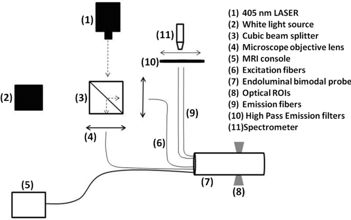
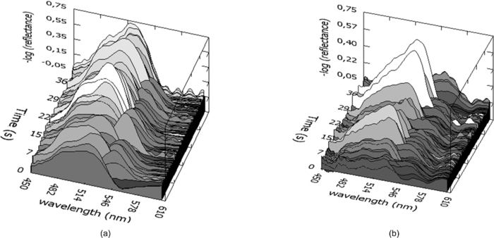
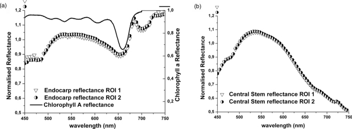
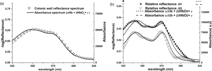
1.

Introduction

Colorectal cancer (CRC) is the fourth most common cancer in men and the third most common cancer in women in the world today.¹ In France, more than 17,400 deaths were estimated for 40,000 new cases detected in 2010.² The 5-year survival rate of all stages combined stands at 56%.³ On the other hand, if the colorectal cancer stages are taken separately, the 5-year survival rate for cases diagnosed at an early stage climbs up to 94%. These figures suggest that an early diagnosis is vital for the life of patients afterwards. But most premalignant lesions develop almost exclusively just underneath the colonic mucosal lining during the early stages, leaving very subtle or practically no morphological changes to the latter. Indeed, colorectal cancer usually develops over a long period of time⁴ (10 to 20 years) and a large majority of CRCs seem to arise from adenocarcinomas.^{5, 6, 7, 8} These subtle or quasi nonvisible changes are very tricky to detect with white light endoscopy (WLE), which is considered as the gold standard and the most widely established diagnostic technique today.^{9, 10}

Nevertheless, over the past decade the ability to miniaturize both optical and electrical components, along with ground-breaking advances in biomedical engineering, have paved the way for different techniques that are rapidly morphing gastrointestinal endoscopy. The emergence of endoscopic techniques,¹¹ such as confocal laser endoscopy¹² and endomicroscopy,^{13, 14, 15, 16} which allow real time high-resolution imaging of cellular and subcellular tissue structures, shows the potentiality of these new techniques. The exciting prospects of optical coherence tomography have also been shown in numerous studies.^{17, 18, 19, 20} Narrow band imaging is another interesting technique that has been in the limelight. The use of special narrow bandpass filters allows the selection of certain wavelengths more than others, and thus helps to greatly enhance the visibility of microvasculature and other subtle tissue structures that are usually invisible with the whole white light spectrum.^{21, 22, 23, 24} Virtual colonoscopy is another different technique which involves the use of magnetic resonance imaging (MRI) or computed tomography to noninvasively scan the patient's digestive system.^{25, 26, 27, 28} After image reconstruction based on surface or volume rendering,²⁹ the gastroenterologist can explore the colon to look for potentially malignant lesions. Optical spectroscopy is a technique which makes use of the interaction of light with tissue. The architectural and biochemical differences between a normal and a cancerous tissue affect the interaction of light with the tissue and produce different spectral signatures in both cases, thus allowing the tissues to be differentiated. Autofluorescence^{30, 31, 32, 33} and reflectance^{34, 35, 36, 37} spectroscopy are techniques that extract these spectral signatures usually using blue light and white light, respectively. Both techniques are currently largely being actively investigated by different groups around the world. MRI,^{38, 39, 40} though less put forward, is also forging its way among the different techniques that provide well-resolved morphological data in the form of images without being invasive and ionizing.

Our approach, in light of all these well-established and emerging techniques, is to combine optical spectroscopy in the form of autofluorescence and reflectance spectroscopy with high spatial resolution magnetic resonance imaging (HR-MRI) within an endoluminal bimodal probe to provide a tool capable of extracting both biochemical data and morphological data simultaneously.^{41, 42} The short term aim of the optical modality is to allow differentiation between a normal tissue and a suspicious or premalignant tissue, with the long term aim being the ability to provide a real-time optical biopsy. HR-MRI, with the aim of allowing a mucosal submucosal complex differentiation, will also assist optical spectroscopy with the high resolution images providing substantial visual support for more accurate interpretation of the spectral signatures.

In this paper, we thus present the conception of the current bimodal endoluminal probe prototype, along with the characterization and the preliminary results that we have obtained both on an organic phantom, the kiwi fruit, and in vivo on a rabbit.

2.

Material and Methods

2.1.

Probe Design

Based on a priori knowledge obtained from a first study dedicated at building a premier macroscopic bimodal prototype, the current prototype was conceived [Figs. 1a, 1b]. The whole probe was designed around a simple-loop magnetic resonance (MR) coil of rectangular geometry already developed and characterized previously.⁴³ The MR part and optical part of the probe were built separately and merged afterwards.

Fig. 1

(a) Schematic diagram of the bimodal probe conceived using Solidworks^®. (b) MRI-optics endoluminal probe used during experiments.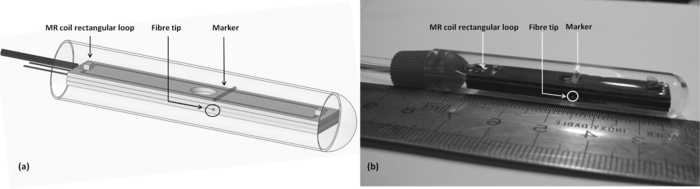

The conductive pathway was designed with a rectangular geometry and was etched by chemical milling on a printed circuit board (PCB) of 50 mm (L) × 10 mm (W) × 0.8 mm (H). Two coils were built for experiments at 1.5 and 3 T. Each coil had a printed circuit assembly composed of a set of case A ATC capacitors (American Technical Ceramic, New York) that allowed a 63.7 and 123.4 MHz tuning frequency, respectively (proton resonance frequency at 1.5 and 3 T magnetic field) and a 50 Ω match for both. An active decoupling circuit was also included using a positive-intrinsic-negative diode driven by the MR system during radio frequency pulse transmission.

The optical part of the probe was crafted on a copper-free PCB of the same geometry and size as the MR coil. Two parallel 800-μm large and 25-mm long grooves with a 9-mm curvature radius at each end were carved on one face of the PCB and each groove sported a pair of fibers. Each pair was composed of a 200 μm core diameter excitation and an emission fiber with a 0.22 numerical aperture (HCG-M0200T Sedi Fibres Optiques, UV-VIS optical fiber). Another rectangular copper-free PCB topped the one with the fibers and double-sided tape was used to fix both. The MR coil imaging structures that are around the probe (lateral imaging), the curved grooves allowed the fibers to be bent and ensure that the region of interest (ROI) of both optical and MR modality was the same. Since two pairs of fibers were used, two optical channels were available for optical acquisitions, with each channel performing measurements on two different sides (left and right) of the probe with respect to their positioning. Thus, this configuration allowed real-time optical differential measurements to be carried out. A 0.8-mm diameter tube filled with 1.25-g/l NiSO₄ water solution was also fixed on the upper face of the PCB in the same plane as the fiber tips and at their exact location. It was used as a marker for precise optical ROI localization on MR images on which it appeared hypercontrasted. Both sets of PCB (optical part and MR part) were fixed together using double-sided tape in the final step. The whole probe was then sheathed in a cylindrical glass tube (ø-12 mm, length, 50 mm).

2.2.

Test Bench

An external optical test bench (Fig. 2) capable of sending and receiving light to and from the probe was designed to perform the optical acquisitions. A 405 nm laser (Roithner Laser, maximum output power of 50 mW) was chosen for autofluorescence spectroscopy. Diffuse reflectance spectroscopy was carried out with a halogen white light source (Zeiss lamp). It should be noted that only one light source was used at a time and thus autofluorescence and reflectance spectroscopy were carried out sequentially. A 6.25 mm cubic beam splitter (NT45–110, Edmund Optics) was coupled to two 20× microscope lenses (Newport Corp, M-20×, 0.4 NA, 9 mm focal length, 1.7 mm working distance) to split, focus, and inject the excitation light into the 2 excitation fibers (200 μm core diameter, 0.22 NA, HCG-M0200T Sedi Fibres Optiques) simultaneously. Two 10 × microscope lenses (Newport Corp, M-10×, 0.25 NA, 16.5 mm focal length, 5.5 mm working distance) were used to focus the emission light on the collecting tip of the spectrometer. A high-pass emission filter (HQ435LP, Chroma Filters) was also added between the two lenses to minimize any residual excitation light. To prevent any cross-talk of the signal from each collecting fiber, the latter were lodged in a specially designed mechanical part which kept them parallel to each other and separated by the fiber overcoating.

Fig. 2

Schematic of the whole setup used for data acquisition.

A multichannel optical system (Specim^® spectrometer coupled to cooled Andor^® Ixon CCD camera with a 6 nm spectral resolution) was used for the in vitro characterization study (on a cylindrical phantom) and a single-channel spectrometer (USB2000 Ocean Optics^® with a 2 nm spectral resolution and typical acquisition time ranging from 100 to 2000 ms) was used in studies on the kiwi fruit and the rabbit's colonic wall. Constructor software along with home-brewed LABVIEW-based programs were used to drive the spectrometers, for focalization purposes, to perform acquisitions, and process the optical data.

As for MR acquisitions, the coil was connected to the MR-console via a coaxial cable and the Siemens flex interface. It should be noted that the optical bench which contained ferromagnetic materials was set up in the MR-console room which is separated from the MR scanner room.

Furthermore, it should be noted that all optical results presented in this work are instrument response function (IRF) free. A calibrated tungsten light source (HL-2000-CAL, Ocean Optics) was used to calibrate the spectral response of both spectrometers (Specim^® and USB2000). The IRF was obtained by dividing the spectral response observed (by each spectrometer) by the expected spectral response curve of the calibrated source provided by the constructor.

2.3.

Validation Steps

2.3.1.

In vitro characterization

The multichannel spectrometer allowed simultaneous acquisition of optical data from both collecting channels, all the while increasing the signal-to-noise ratio (SNR). Dynamic acquisitions from both channels while moving the probe was also possible. LABVIEW-based programs were used to optimize light focalization of the collecting fibers on the spectrometer and to process the raw data after acquisition.

The home-built cylindrical phantom (Fig. 3) used consisted of two identical 1-mm inner diameter flexible transparent tubes (clinical catheters produced by CAIR LGL Company, ref PB3110M) that were twirled around each other. The tube being transparent, its absorption and diffusion coefficients were thus negligible with respect to any nontransparent material. A transillumination experiment (results not shown) was carried out to confirm that the optical properties of the flexible transparent tube did not significantly affect the optical properties of the contrast agents (rhodamine and eosin). We therefore considered that it did not impact on the optical properties (absorption and diffusion) of the eosin and rhodamine B solutions. The resulting hollow cylindrical tube was enfolded in a thin transparent plastic film to maintain both tubes together as well as the cylindrical form of the phantom. A 20 μmol/l rhodamine B solution (using pure ethanol) was injected in one of the tubes. Another solution made of 0.3 mmol/l of eosin and 2.2 mmol/l of gadolinium (using pure ethanol) was injected into the other tube of the phantom. Gadolinium at that concentration reduced the T₁ (longitudinal) relaxation time of the eosin solution to 150 ms and allowed the latter to appear in hypercontrast compared to the rhodamine B solution on T₁-weighted MR images, and thus visually differentiate the two tubes containing the two different fluorophores.

Fig. 3

Home-built phantom consisting of two 1 mm inner diameter flexible tubes twirled around each other. Each tube was filled with a 0.01 g/l rhodamine B solution and 0.2 g/l eosin solution, respectively. Gadolinium was also added in the tube containing eosin.

Measurements were carried out at 1.5 and 3 T on Siemens Avanto and Verio clinical MR system, respectively. The probe was inserted inside the phantom without using any aqua gel (the aperture being sufficiently large for the probe to slide inside with ease and be in direct contact with the tubes) and acquisitions were made for two fixed positions. For the optical part, for each fixed position of the probe within the phantom, autofluorescence, and reflectance acquisitions were carried out. White paper was used as the reference sample in reflectance measurements. The latter was folded around the probe (to keep the same form as the test sample) during each reference reflectance spectrum measurement. It was ensured that no spectral distortion was induced by the reference sample through preliminary measurements where the reflected light spectrum (by the paper in experimental conditions) was compared to that of the incident light (white light source) and no significant difference was observed. Intensity of the white light was constantly monitored (direct measurement through an optical fiber placed between the light source and the spectrometer) and compared to the reference light acquired from one measurement to the other. As for exposition times used, they were typically on the order of 250 to 1500 ms. The optical power per excitation channel was fixed at 1 mW for autofluorescence measurements using the laser light. A halogen white light (Zeiss lamp) at 3250 K was used for reflectance measurements. Background correction was systematically carried out for every optical acquisition made. These parameters allowed a good SNR while avoiding any photobleaching effect. During autofluorescence acquisitions, the white light source was shielded instead of being switched off, and for reflectance acquisitions the laser light source was shielded. This ensured that the photon flux from the excitation sources remained steady in between two measurements and that the latter were afterwards comparable.

Dynamic autofluorescence and reflectance measurements during which the probe was moved at an average speed of 3 mm/s were also performed on a given length (10 cm) of the phantom. Optical exposure times were carefully chosen with a maximum of 250 ms/spectrum to minimize any spectral overlapping of the signal emitted by rhodamine B and eosin, respectively, while the probe was moved within the phantom. It should be noted that the optical acquisitions were synchronized on the MR scans carried out simultaneously. Comparing optical data to MR data was thus more precise.

To further the study, the cylindrical phantom was replaced by a kiwi fruit and the same experimental procedure was repeated at 1.5 T.

2.3.2.

Organic sample

Technical validations and system efficiency tests were carried out on a kiwi fruit on a 1.5 T Siemens Sonata clinical MR system. The kiwi was an excellent test sample since its high water content provided high signal intensity during MR acquisitions and allowed the finely detailed structures of the fruit to be visualized while the important chlorophyll concentration produced a characteristic autofluorescence signature.⁴⁴ Moreover, the kiwi was ideal to perform differential measurements and diffuse reflectance spectroscopic measurements owing to its green endocarp and central white stem which could be analyzed simultaneously by each optical channel of the probe.

Before acquisition, the fruit was laid on the MR scanner bed and the endoluminal probe was inserted inside in such a way that the optical ROI of each optical channel was the green endocarp and the central white stem, respectively. The scanner bed was then moved 80 cm inside the scanner itself for both MR and optical acquisitions. Several MR sequences (Flash, True-Fisp, 3D True-Fisp, Turbo-Spin Echo) were used in transverse and coronal orientation planes with different weighted contrast (proton density-, T₁-, T₂-, T₂*-weighted).

Each optical modality (autofluorescence and reflectance) was tested on the two different ROIs. Exposure times of 300 and 600 ms were used for autofluorescence acquisitions while for reflectance measurements, exposure times of 600 and 900 ms were chosen. As in the study on the cylindrical phantom, paper was used here over as a reference material for reflectance measurements.

2.3.3.

In vivo experiment on a rabbit

The whole setup was tested in vivo on a healthy New-Zealand white rabbit in another study following the promising results obtained on the kiwi fruit. Results presented in this study are mainly intended to demonstrate the proof of concept and feasibility of such a technique in vivo explaining the use of only one rabbit in this study. Moreover, know-how and knowledge acquired through previous HR-MRI studies⁴³ on a group of rabbits were put forward to enhance our interpretation of the results. All testing strictly abided to an animal protocol (protocol number BH2010–26) that had been approved by the university ethic committee. The rabbit was anesthetized prior to any intervention. An aqua-gel that was verified to be free of any fluorescent characteristics at 405 nm (to ensure that no parasitic fluorescence resulted from the aqua gel itself) was used to facilitate the probe insertion. The probe was inserted 10 cm inside the colon. The optical setup used was unchanged as was the optical power per excitation channel. Acquisition times for optical measurements varied from 250 to 2000 ms. Both optical and MR data were collected simultaneously. A pre-established imaging protocol composed of different high-resolution sequences (2D FLASH, 3D True-Fisp, turbo spin-echo) was used for MRI. Basic imaging parameters ranged from 60 to 80 mm for the field of view (FOV), 1.5 to 2.5 mm for slice thickness and 256 to 448 base matrix for encoding. Three different ROIs were arbitrarily chosen and analyzed. For each ROI, the autofluorescence and reflectance spectrum were acquired along with the MR scans. Additionally, for the third ROI, dynamic reflectance acquisitions were performed. We also show that endoluminal coil tracking which allows spatial localization of the probe within the rabbit's colon is possible with a coronal two-dimensional (2D) True-Fisp sequence and real time reconstruction with an image/s acquisition rate.

3.

Results

3.1.

In Vitro Characterization

Time constraints restricted our optical acquisitions to fluorescence and reflectance measurements at two fixed positions of the probe within the cylindrical phantom and a single series of dynamic fluorescence measurements on the 3 T clinical MR scanner.

MR results of a T₁ FLASH 3D sequence (flip angle of 15°, TR/TE of 11/3.7 s; 12 × 12 cm FOV; 320 × 320 matrix) provided the maximum intensity projection (MIP) image shown in Fig. 4a. The eosin-gadolinium solution present in one of the two tubes appears in hyperintensity compared to the rhodamine B solution in the other tube. While illustrating the difference in contrast between the eosin-gadolinium solution and the rhodamine B solution, Fig. 4b which is a single MR slice from the T₁ FLASH 3D sequence, also shows the exact location of the optical channels (white arrows) through the water-filled marker which appears hypercontrasted.

Fig. 4

(a) MIP image of the cylindrical phantom obtained with a T1 Flash 3D sequence at 3 T. Eosin-gadolinium solution appears hyper contrasted compared to rhodamine B solution. (b) Example of a single MR scan of the cylindrical phantom obtained with the T1 Flash 3D sequence. The hypercontrasted rectangular zone in the middle of the image corresponds to the water-filled marker.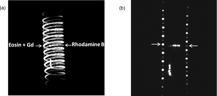

Autofluorescence results [Fig. 5a] obtained for this particular position of the probe within the phantom correlated well with the MR scan of Fig. 4b. Fluorescence intensity of the eosin+Gd solution was 35 times higher than that of rhodamine B. The eosin+Gd fluorescence curve peaked at 555 nm, while that of rhodamine had a maximum at 575 nm and was heavily polluted by the parasitic fluorescence of the plastic tube (results of the fit are not shown) in the 450 to 525 nm bandwidth. Though the plastic tube used in the phantom was completely transparent and did not affect reflectance measurements directly, autofluorescence measurements carried out on the plastic tube alone showed that it emitted a fluorescence signal, which in our case was parasitic and affected the rhodamine fluorescence spectrum.

Fig. 5

(a) Comparison of the left and right ROI fluorescence spectra obtained on the cylindrical phantom. Eosin fluorescence was observed at 555 nm and rhodamine B at 575 nm. (b) Comparison of the left and right ROI reflectance spectra obtained on the cylindrical phantom. Reflectance spectrum of rhodamine B peaked at 547 nm while that of eosin + Gd was less clear-cut.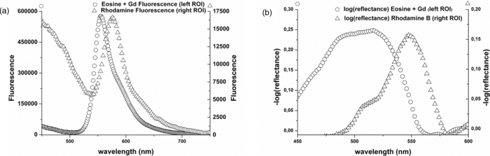

The eosin+Gd reflectance curve [Fig. 5b] was significantly distorted in the 450 to 525 nm bandwidth while the rhodamine B reflectance curve peaked at 547 nm and was quasi not affected in the same spectral bandwidth. Reflectance spectrum of the plastic tube used to build the phantom was also measured and fitting (fit not shown) the eosin+Gd reflectance spectrum with a combination of pure eosin+Gd reflectance spectrum and pure plastic reflectance spectrum produced similar results (results not shown).

It is worth remembering that eosin was used in a concentration 20 times higher than that of rhodamine B. The absorption coefficients of both solutions were determined (a specific experiment not detailed in this study was carried out for that purpose) and the eosin solution had an absorption coefficient of 41 cm⁻¹ at its maximum absorption wavelength (523 nm in our case), while the rhodamine B solution had an absorption coefficient of 6 cm⁻¹ at its maximum absorption wavelength (542 nm in our case).

Dynamic acquisitions during which the probe was moved over a determined length (5 cm) within the phantom while both MR and autofluorescence measurements were made yielded the results presented in Figs. 6, 7, respectively. Only 3 MR images out of 30 acquired from this T₁ FLASH 2D sequence are shown. The contrast between the eosin-Gd solution and the rhodamine B solution can easily be distinguished and the different positions of the water-filled marker once again clearly show the different ROIs analyzed by the optical channels. These ROIs varied both for the left and right channel since the probe was being moved and the position of the marker was thus used post-acquisition to correlate the images to the different measured spectra.

Fig. 6

Example of images acquired during dynamic acquisitions with a T1 FLASH 2D sequence. The probe was moved within the phantom and the marker's position allowed optical results to be correlated to the MR images.

Fig. 7

Dynamic autofluorescence acquisitions of the left and right optical channels. Two different curves corresponding to fluorescence emitted by the eosin-Gd solution and the rhodamine B solution can clearly be observed along with the alternating pattern while the probe is moved.

The autofluorescence results (Fig. 7) obtained shows an expected alternating pattern between the eosin-Gd spectrum and rhodamine B spectrum as the probe was moved. Since the maximum fluorescence intensity of the eosin-Gd solution was 35 times higher than that of the rhodamine B solution, the dataset presented here over have been normalized and an optimized Savitzky–Golay filter⁴⁵ (inducing no spectral distortion) applied to better highlight this interchanging pattern. This changing pattern can also be observed between the left and right acquisition channel.

The same study was also carried out using a 1.5 T clinical MR scanner. The MIP volume presented in Fig. 8a was obtained using the same T1 FLASH 3D sequence (with identical parameters) used at 3 T. This step validated the good functioning of the endoluminal probe at the two most widely used clinical MR fields (1.5 and 3 T) nowadays.

Fig. 8

(a) MIP volume of the cylindrical phantom obtained with a T1 Flash 3D sequence at 1.5 T. (b) MIP volume of the cylindrical phantom obtained with a T1 Flash 3D sequence at 3T.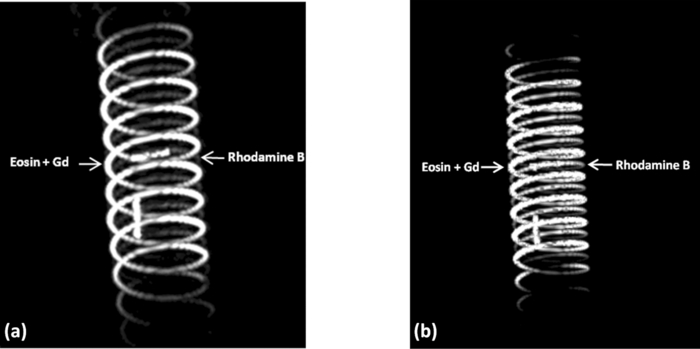

Fluorescence and reflectance results obtained (results not shown) for the fixed positions of the probe within the phantom were identical to those of the same study at 3 T (presented in Fig. 5). Dynamic reflectance spectroscopic acquisitions were also made while moving the probe within the phantom. The reflectance spectra obtained from these measurements for both eosin-Gd and rhodamine B correlated well with the spectra obtained for fixed positions of the probe within the phantom. Figures 9a, 9b show the interchanging pattern observed for reflectance measurements made on the left and right ROIs, respectively. Eosin-Gd solution's reflectance curve had a significantly lower amplitude compared to rhodamine B's reflectance curve as it can be observed on the dynamic sequence of the left and right ROIs presented in Figs. 9a, 9b, respectively. The reflectance spectrum of rhodamine B was, however, still heavily affected by specular reflectance in the 450 to 500 nm bandwidth.

Fig. 9

Dynamic reflectance acquisitions made by the left optical acquisition channel (a) and the right optical channel (b) of the endoluminal probe on the cylindrical phantom. Rhodamine B's reflectance curve is heavily polluted by specular reflectance of the plastic tube.

3.2.

Organic Sample

The above MR image of the kiwi fruit with an SNR of 25 was obtained with the MR coil of the bimodal endoluminal probe in study 1. A T₂*-weighted FLASH 2D sequence with a 40 deg flip angle, a TR/TE of 650/18 ms, an 80 mm FOV, a 2 mm slice thickness, and 256 × 205 matrix was used. The fine structural details such as the seed coats and the capillaries linking the pericarp to the central stem of the fruit can clearly be observed. The endocarp can also be clearly distinguished from the central stem. The doped-water filled tube used as a marker appears hypercontrasted at the center of the MR image and points to the exact location (represented by the black brackets in Fig. 10) of the two optical ROIs. During this sequence in which the probe was in a fixed position, the MR scan shows that the left and right optical channels were positioned on the endocarp and the central stem, respectively.

Fig. 10

MR image of kiwi fruit in study 1 with a T₂*-weighted FLASH sequence; TR/TE: 650/18 ms; 80 mm FOV; 2 mm slice thickness; 256 × 205 matrix.

Autofluorescence [Figs. 11a, 11b] spectra of the green endocarp were compared to those of the central white stem. A characteristic peak⁴⁴ at 680 nm was observed both in the endocarp and the central stem with the former having a higher intensity for the same exposition time. The central stem also exhibited noticeable fluorescence between 450 and 600 nm compared to the endocarp. The ratio of the area under the curve between the 450 to 600 nm interval and the 650 to 750 nm interval was calculated for the endocarp and the central stem, respectively. The values ranged from 42 to 60 for the former and 3.5 to 4.5 for the latter.

Fig. 11

(a) Fluorescence spectra of three different ROIs on the green endocarp of the kiwi fruit obtained with three different exposure times and 405 nm excitation light. (b) Fluorescence spectra of three different ROIs on the central white stem of the kiwi fruit obtained with three different exposure times and 405 nm excitation light.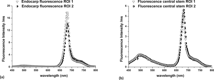

The diffuse reflectance spectrum of the green endocarp differed significantly from that of the central white stem [Figs. 12a, 12b]. In the blue region, up to 475 nm, reflectance was low for the endocarp [Fig. 12a]. In the green-yellow bandwidth reflectance increased and then gradually decreased in the orange region with a sharp drop in the red bandwidth, more precisely near 650 nm which corresponds to the region of high absorption by chlorophyll a.^{46, 47} Reflectance then underwent a steep rise until 680 nm, followed by a sudden drop over the next 50 nm. Maximal and almost invariable reflectance was observed as from 725 nm in the endocarp of the kiwi fruit. In contrast, the central white stem exhibited a more monotonous reflectance spectrum with a gradual rise from 450 to 520 nm and peaking at 525 nm followed by a steady decrease until 750 nm. The steep rise observed at 680 nm in the reflectance spectrum of the endocarp was absent in that of the central white stem.

Fig. 12

(a) Normalized reflectance spectra of three different ROIs on the endocarp of the kiwi fruit. Absorption spectrum of chlorophyll A is also shown for comparison. (b) Normalized reflectance spectra of three different ROIs on the central white stem of the kiwi fruit.

3.3.

In vivo Experiment on Rabbit

Real-time tracking of the endoluminal probe within the colon was also performed. The MR console automatically combined images obtained by an external coil with those obtained by the endoluminal probe and provided MR scans where the probe was clearly visible. The image batch obtained from the MR sequence allowed continuous tracking of the probe. Only two positions are shown in the example below. The doped water-filled marker which appears hypercontrasted on the image (white arrows in Fig. 13) was our marker to localize both the probe and the optical channels.

Fig. 13

Real-time endoluminal coil tracking allowing precise spatial localization of the optical probe and the optical channels using the water-filled marker which appears hypercontrasted. A 2D True-Fisp sequence and real-time construction with a 1 s/image acquisition rate produced these images.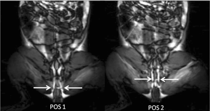

The contours of the mucosal and submucosal complex were clearly distinguishable [Fig. 14a] on the high-resolution MR images obtained with the endoluminal coil using multislice transverse HR-MRI. The same ROI was also imaged using the external coil and while applying strictly the same parameters and imaging sequence, the resulting images obtained did not allow any distinction between the mucosal and submucosal complex [Fig. 14b]. The SNR gain of the endoluminal coil versus the external coil measured at 15 mm from the center of the image (white circle in Fig. 14) was still of 25/1 in favor of the endoluminal coil. As for the marker on the MR scan [hypercontrasted zone in the middle of the MR image of Fig. 14a], it allowed us to locate the optical ROI analyzed and compare the morphological information to the biochemical information

Fig. 14

MR image obtained with the endoluminal coil (a) and an external coil (b) both with the same T₂-weighted TSE sequence. SNR gain of the endoluminal coil/external coil measured at 15 mm from the center of the image (white circle) was 25/1.

Optical acquisitions were also carried out on two different ROIs both for the left and right acquisition channels. The autofluorescence spectra of two different ROIs are presented in Figs. 15a, 15b, with the latter being compared afterwards to the corresponding MR scan [Fig. 14a]. Data presented have been normalized by the acquisition time. The first zone of analysis composed of ROI 1^′ and ROI 2^′ [Fig. 15a] exhibited a fairly similar fluorescence spectrum. Maximum fluorescence intensity was observed in the 450 to 525 nm bandwidth with both curves peaking at 480 nm. Two relatively small shoulders were also observed at 625 and 675 nm.

Fig. 15

(a) Fluorescence spectra acquired with the endoluminal probe. ROI 1^′ and ROI 2^′ were analyzed by the left and right optical channel, respectively. (b) Fluorescence spectra acquired with the endoluminal probe. ROI 1 and ROI 2 differ from ROI 1^′ and ROI 2^′ as the probe was moved to another position. Fluorescence spectrum of the rabbit's faeces is also represented here.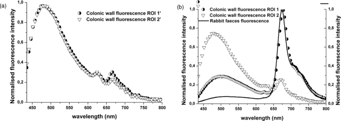

ROI 1 and ROI 2 [Fig. 15b], which formed the second zone of analysis, exhibited different fluorescence spectrum each. The spectrum emitted by ROI 1 and ROI 2 in the 450 to 625 nm bandwidth differed while ROI 1 showed pronounced fluorescence emission at 675 nm. The rabbit's faeces fluorescence spectrum was also acquired [represented in Fig. 15b] and it fitted ROI 1's spectrum perfectly in the 650 to 750 nm bandwidth [Fig. 15b]. This also confirmed its suspected influence on the fluorescence spectra as in Fig. 15a (shoulders observed at 675 nm). A more general fit was also tested on the whole spectral band (for ROI 1) using fluorescence data of the faeces and of the colonic wall, respectively. Results obtained once again fitted ROI 1's spectrum perfectly on the whole spectral band and also explained the spectral shift on the right observed in the 450 to 600 nm band.

The reflectance spectra obtained on the different ROIs were relatively similar in form. One of these spectra is presented in Fig. 16a. From 450 to 500 nm, there is relatively high reflectance. In the 500 to 600 nm range, pronounced absorption was observed. The reflectance spectra were fitted with Hb and HbO₂ absorptivity values.⁴⁸ A simple modified Beer–Lambert's law under the form of αHb + ßHbO₂+ γ was used as a first approximation for fitting. A series of dynamic reflectance acquisitions lasting 50 s, during which a spectral measurement was made every 5 s, was also performed on a fixed ROI. The variation of each spectrum (relative reflectance) with respect to the first acquired spectrum in the series was then calculated. Two of those relative reflectance spectra are presented in Fig. 16b and fitted with Hb and HbO₂ absorbance values following the equation stated above. α and ß, which are the coefficients used to ponder Hb and HbO₂, varied for each fitted spectrum. They were of 48% and 52% for the spectrum measured at time interval t ₁ [Fig. 16b] and of 54% and 46% for the spectrum measured at time interval t ₂ [Fig. 16b].

Fig. 16

(a) Reflectance spectrum of the rabbit's colonic wall (ROI 1^′). Spectrum was fitted with Hb and Hb0₂ absorptivity data. (b) Relative reflectance spectra of ROI 1^′. Each spectrum was divided by the first measured spectrum in the series and fitted with sets of Hb and Hb0₂ absorptivity data.

4.

Discussion

The eosin and rhodamine B solution which were in two distinct plastic tubes were clearly differentiable on the MR images acquired at 1.5 and 3 T. Protons in the eosin-gadolinium solution had a relatively shorter T₁ relaxation time (which differed at 1.5 and 3 T) compared to the protons of the rhodamine B solution due to the presence of the gadolinium complex,⁴⁹ and this characteristic created a fine contrast on the MR images. This contrast was much more highlighted on MR images at 1.5 T because of the difference of T₁ values between eosin and rhodamine B solution being more significant at 1.5 T than at 3 T. Indeed, T₁ values generally tend to be longer as the magnetic field gets higher, and thus the difference between short T₁ values and long T₁ values is reduced, provoking a less marked contrast between two samples for example.⁵⁰ This can easily be observed on the MIP image of the cylindrical phantom at 3 T [Fig. 8b], where a much smaller contrast ratio is observed compared to the MIP image at 1.5 T [Fig. 8a].

The single MR scans with the hypercontrasted marker gave the exact location of the optical channels each time within the phantom and allowed us to correlate the optical spectra to the MR scans. Fluorescence spectra of both eosin-Gd solution and rhodamine B solution showed different peak shifts when compared to spectra found in the literature, and these studies tend to show that a spectra shift might be the result of concentration or temperature differences.^{47, 51, 52, 53} However, both eosin and rhodamine showed distinct peaks at 555 and 575 nm, respectively. Fluorescence spectra of eosin-Gd solution were negligibly affected by the parasitic fluorescence emitted by the plastic tube of the phantom compared to the spectra emitted by rhodamine B. The quantum yield of both eosin and rhodamine B solutions being relatively similar, the 20-fold difference in concentration between the two solutions is the main criteria accounting for this phenomenon. Indeed, the intensity of the fluorescence emitted by eosin is 34 times higher than that of both rhodamine and the plastic tube (fluorescence spectrum measured in a different experiment and results are not shown). Any fluorescence emitted by the latter is thus masked or negligible compared to that of eosin's and does not affect its spectrum. On the other hand, the fluorescence intensity of rhodamine B and the plastic tube being of the same order of magnitude, the resultant spectrum is distorted by the spectral signature of the plastic tube. Fitting the empirical data with the pure spectra of rhodamine B and plastic tube, respectively, confirms this hypothesis (results not shown).

A similar phenomenon was also observed on the reflectance spectra. However, it occurred on the opposite solutions this time compared to the fluorescence spectra. The eosin reflectance curve was heavily distorted by the specular reflection on the plastic tube while that of rhodamine B was quasi unaffected. It is worth remembering that eosin was used in a concentration 20 times higher than that of rhodamine. Moreover, the ratio of the absorption coefficients at maximum absorption wavelength (41 cm⁻¹ for eosin at 523 nm and 6 cm⁻¹ for rhodamine B at 542 nm) for the two solutions is of 7:1. This implies that the number of photons (from the white light excitation source) absorbed by eosin is significantly higher than those absorbed by rhodamine B. In other words, the number of photons reflected back by eosin is significantly less compared to rhodamine B, and the specular reflection of the plastic tube is much more present in the 450 to 500 nm bandwidth of the eosin reflectance spectrum than in rhodamine's.

Optical dynamic acquisitions carried out at 3 and 1.5 T did not show any difference. This validates the fact that there is no interference of the magnetic field on the optical measurements, whatever the field value (between 1.5 and 3 T). Moreover, the fluorescence curves clearly show that the optical channels of the bimodal endoluminal probe are able to measure fluorescence emission of at least two different fluorophores within short acquisition times. The fluorescence curves on the three-dimensional (3D) graphic were normalized to highlight the interchanging pattern, while the probe was moved within the phantom. This maneuver also highlights the parasitic effect of the plastic tube fluorescence on the rhodamine spectrum. Being able to measure different spectra with the left and right channels provide each time two different ROIs with either the same or different spectral signatures. This important characteristic can be used for comparison purposes in future in vivo studies and facilitate differentiation between tissue states.

As for the dynamic reflectance spectra acquired and presented on the 3D graphic of Fig. 9, the interchanging pattern of the measured spectrum while the probe was moved can still be observed. The data clearly show the distorted spectrum of eosin due to specular reflection compared to rhodamine B. The impact of this parasitic signal can, however, be considered as negligible on the expected results. Indeed, the spectral signature of the plastic tube being known and the optical system being able to acquire and differentiate the signal emitted by each fluorophore, the expected results can still be retrieved by fitting the data. This important point should be taken into account in future studies in order to avoid any signal masking by parasitic emission.

Concerning the results obtained on the organic sample, the different structures ranging from the pericarp to the central stem of the kiwi fruit (actinidia) were clearly visible on the MR images obtained with the endoluminal coil at 1.5 T. A planar spatial resolution of 310 μm allowed these fine details to be observed. However, a better in-plane spatial resolution (up to ∼150 μm) is still achievable with the endoluminal probe by optimizing the acquisition parameters, the downside remaining an increased acquisition time.

As for the optical results, the fluorescence emission peak observed at 680 nm for the pericarp is characteristic of photosystem II antennae⁴⁴ and corresponds to fluorescence emitted by chlorophyll a. The shoulder appearing with a much lower intensity between 730 and 740 nm seems to be typical of the photosystem I antenna. This significantly lower intensity indicates a reduction in size of the photosystem I antenna chlorophyll as it has been suggested in the literature. As for the central white stem, the same characteristic peak at 682 nm was also observed but the fluorescence curve showed additional fluorescence between 450 and 600 nm compared to fluorescence emitted by the pericarp. The origin of this fluorescence may possibly come from the family of carotenoids⁵⁴ present in non-negligible concentrations compared to chlorophyll in the central white stem; the area under the curve ratio between 650 and 725 nm and 450 and 550 nm bandwidth is of 42 for the pericarp and of 5 for the central stem. The presence of carotenoids has not been investigated, the initial aim of the study being a feasibility study. However, this difference between the pericarp fluorescence and the central white stem fluorescence was used as a differentiation criterion between these two structures, and the good correlation with the MR images each time provided further proof of the correct optical analysis. It is worth noting that illuminating the Chinese gooseberry with a 405 nm laser light and observing the fruit through a pair of 450 nm high-pass filtering goggles clearly highlights the pericarp which appears red and a much more contrasted whitish green central stem.

The reflectance spectra acquired provided additional information which, when correlated to the fluorescence spectra, allowed us to distinguish the pericarp from the central stem even before comparison with MR images. The reflectance curve of the pericarp was compared to the absorbance curve of chlorophyll a and the sharp drop around 662 nm fairly coincided with the high absorption shown by the latter in that bandwidth. This underlines the high concentration of chlorophyll a present in the kiwi's pericarp. Moreover, the steep rise in the 665 to 682 nm with a maximum at 684 nm seems to correspond to autofluorescence of chlorophyll a stimulated by the white light used for the reflectance measurements. These characteristics have previously been reported in the literature though not specifically on the kiwi fruit.⁴⁶ The central stem emitted a rather different reflectance spectrum with a gradual and continuous decrease reflectance from 550 to 750 nm and no manifest stimulated autofluorescence of chlorophyll in the 665 to 682 nm bandwidth. These observations tend toward concluding that chlorophyll concentration in the central white stem was seemingly lower compared to the pericarp's and any fluorescence emitted was possibly masked or insignificant.

For the study carried out in vivo on the rabbit with the endoluminal bimodal probe, MR results obtained had a far better SNR compared to those obtained with an external coil. The compactness of the probe, which was rendered possible by the geometry of the MR coil, allowed contact with the tissue to be analyzed and thus drastically increased the SNR. The colonic mucosa submucosa complex was clearly distinguishable with a planar resolution of 155 μm that was achieved with the endoluminal coil. This is worth noting because such clear differentiation will be of utter importance in future studies of a cancer model. Indeed, such high SNRs cannot be achieved by the external coils and thus the mucosal and submucosal complex, which is the preferential site of cancer development in the colon, cannot be clearly differentiated.

As for fluorescence results, the main fluorophores that were excited in the 450 to 600 nm range coincide with NADH fluorescence observed in vivo on human esophageal tissue,⁵⁵ thus suggesting the presence of NADH within the rabbit's colonic tissue. Moreover, fluorescence spectrum of the rabbit's faeces was also acquired and compared to the spectra obtained within the rabbit's colon. The peak appearing around 665 nm in the colonic wall fluorescence of ROI 1^′ and ROI 2^′ which seemed to coincide with that of the rabbit's faeces, suggesting the presence of the latter within the optical field of view was confirmed by the MR scans (results not shown). The rabbit's faeces fluorescence curve also coincided with that of chlorophyll a and this can be explained by the fact that the rabbit followed a Teklad Global Rabbit diet, and the main ingredient was dehydrated alfalfa which contains chlorophyll. Moving the probe to a different zone of analysis provided the fluorescence results of Fig. 11b (ROI 1 and ROI 2). Results of ROI 1 were heavily affected and distorted by fluorescence of the rabbit's faeces which were present in the optical field of view and clearly visible on the corresponding MRI slice. ROI 2 was, on the other hand, a zone that contained no faeces as suggested the corresponding fluorescence curve, and this was also clearly visible on the corresponding MRI slice.

Reflectance data obtained on one of the faeces-free zones showed important activity in the 500 to 600 nm range. Fitting the empirical data with absorptivity data of oxy and deoxy-hemoglobin by applying modified Beer–Lambert's law as stated before confirmed the important absorption of the excitation light in the 500 to 600 nm bandwidth and the fact that the colonic wall is highly vascularized. The dynamic acquisitions carried out on the same ROI put in the limelight the varying oxygen saturation in the blood vessels along with the blood volume throughout the acquisitions and also confirmed that the spectra observed were effectively due to hemoglobin. Furthermore, these hemodynamic variations can be simultaneously monitored and compared for two different ROIs through the two different optical channels.

Optical measurements made throughout these different studies never exceeded 5 min. For future in vivo studies this point is fundamental since it will allow quick analysis with both modalities. The ability to make acquisitions while moving the probe is also a real advantage in that it will considerably speed up acquisitions all the while allowing deeper analysis. However, analysis depth is currently limited to 30 cm because it involves security issues related to heating that is induced by radio frequency electric field concentrations in the presence of conducting wires. This is currently being investigated.^{56, 57} Another point to be noted is that MR results were available immediately, while optical spectra were obtained after post-processing. For the time being this is quite difficult since correlation between MRI results and optical results cannot be carried out in real time, but home-brewed LABVIEW-based programs are currently underway to process optical raw data and display them in real-time simultaneously to MRI results.

5.

Conclusion

Following the results obtained, it can be said that a fully functional bimodal endoluminal probe combining HR-MRI to optical spectroscopy has been conceived, fully characterized, and successfully tested. It has been validated on a phantom, a fruit, and in vivo on a rabbit. The next steps involve building a smaller flexible probe with an ideal size (6-mm diameter) for in vivo measurements on small animals and extending the studies to a larger group of animals with predefined colorectal tumor models.