1.

Introduction

Many tissue types, including bone, muscle, skin, and white matter in the brain, have orientated internal structures such that the degree of optical scattering depends on the direction of light propagation. The spatial-dependence of the bulk (e.g., multiple) scattering intensity in these tissues is determined by their microscopic structure. Imaging the directionality of multiple light scattering may provide a noninvasive way to interrogate tissue microscopic structure, and may aid in the early detection and diagnosis of disease.

The orientational dependence of multiple light scattering from ordered structures has been measured in biological tissues including bovine tendon,¹ chicken breast,² skin,^{3, 4} bone,⁴ muscle,⁵ and dentin.⁶ It has also been tested in tissue phantoms.^{7, 8, 9} Researchers have modeled multiple scattering from ordered structures using Monte Carlo simulations of radiative transport,¹⁰ as well as random walk^{11, 12} and finite element implementations¹³ in the diffusive regime. In all of these studies, the emphasis has been to determine the orientation of large homogeneous scattering regions by looking for elliptical equal intensity profiles of the backscattered or transmitted light from a localized (e.g., point) source. Greater eccentricity of the ellipse indicates a higher degree of scattering structure, and the orientation of the ellipse gives the direction of the underlying structure. Such measurements of scattering orientation give the average scattering properties over an area of a few centimeters. This concept is similar to the classical scattering anisotropy, g, which describes the average cosine of the scattering angle over a single scattering length (ℓ), while scattering orientation applies to multiple light scattering based on length scales that are on the order of the transport scattering length, ℓ* ∼ ℓ/(1 − g).

Spatial frequency domain imaging (SFDI) is a wide-field method which measures the absorption and scattering properties of turbid media such as biological tissue.^{14, 15} It combines CCD camera-based imaging with diffuse optical methods in order to simultaneously determine the spatially varying optical properties throughout a sample. Instead of scanning a collimated source beam across the sample, optical properties at each detection location are determined simultaneously by measuring the attenuation of sinusoidal patterns of light which are projected onto the sample at varying spatial frequencies. SFDI has been used to quantitatively image stroke,¹⁶ brain injury,¹⁷ cortical spreading depression,¹⁸ layered structures in skin,¹⁹ and depth resolved fluorescent signals.²⁰ It has also been used to perform tomographic imaging,^{21, 22} detect inhomogeneities,²³ and determine optical properties over a broad range.²⁴

In this manuscript, we use SFDI to image spatially varying scattering orientation in highly scattering media. We begin by deriving a solution to an anisotropic diffusion equation in the spatial Fourier domain. The solution predicts that in turbid media, the attenuation of the projected sinusoidal patterns depends on the orientation of the projected patterns with respect to the subsurface scattering structures. When orientated along the same direction as the underlying scattering structures, the sinusoidal patterns attenuate more quickly with increasing frequencies. If the scattering structures are not parallel or orthogonal to the surface, there is a phase shift of the projected patterns. By rotating the projection patterns and measuring their attenuation and phase shift, we image the spatially varying orientation over a large field of view, and determine the relative direction of the underlying light scattering structures. We also introduce a contrast function, the scattering orientation index (SOI), that describes the degree of scattering orientation independent of other factors such as the overall amount of light scattering and absorption, both of which may also vary spatially. We validate our method using tissue simulating phantoms with fibrous structures, and with ex vivo samples of muscle and brain.

2.

Theory

The propagation of light in turbid media is well described by the radiative transport equation (RTE) which appears as:

Heino et. al. solved Eq. 3 numerically using finite element methods. Here we show that for simple geometries and homogeneous optical properties, Eq. 3 can be solved analytically by decomposing the Greens function into plane waves as has been done for the isotropic diffusion equation.^{21, 27, 28} In the semi-infinite and slab geometries, there is translational invariance along the medium's surface. Let the surface of the diffusive medium be in the x-y plane, and let z represent the depth from the surface. Accordingly we can write Greens function as

Fig. 1

Schematic of the experimental geometry. Gray rectangles represent cylindrical light scattering structures in a turbid medium. Left: top view of the medium where φ is the angle in the x-y plane between the wave number q of the sinusoidal illumination pattern, and the projection of the cylindrical structures onto the x-y plane. Right: side view of the medium where θ is the angle between the surface and the cylinder direction.

Fig. 2

Plot of the calculated amplitude of remitted light as a function of the angle φ between the wave number of the projected sinusoidal pattern, and the direction of the cylindrical scattering structures. The amplitudes due to 5 projection frequencies ranging from 0.1 to 0.5 mm⁻¹ are shown. The minimum occurs when the wave number is aligned with the scattering structures. Higher frequencies are more sensitive to anisotropy, but have smaller average amplitude.

3.

Methods

3.2.

Data Analysis

For each projection angle, the amplitude of the remitted light at every detector location was calculated according to

Eq. 20

[TeX:] \documentclass[12pt]{minimal}\begin{document}\begin{eqnarray} A(x,y) &=& \frac{{2^{1/2} }}{3}\{ {\rm }\left[ {I_1 (x,y) - I_2 (x,y)} \right]^2 + \left[ {I_1 (x,y) - I_3 (x,y)} \right]^2\nonumber\\ && + \left[ {I_2 (x,y) - I_3 (x,y)} \right]^2 \}^{1/2}. \end{eqnarray}\end{document} $$\begin{array}{ccc}\hfill A(x,y)& =& \frac{2^{1/2}}{3}\{{\left[I_1(x,y)-I_2(x,y)\right]}^2+{\left[I_1(x,y)-I_3(x,y)\right]}^2\hfill \\ & & {+{\left[I_2(x,y)-I_3(x,y)\right]}^2\}}^{1/2}.\hfill \end{array}$$

We have discussed this demodulation and the measurement of the amplitude previously.¹⁴ The phase shift of the projected wave can also be calculated,³¹ and has been used for tomographic imaging.²¹ However, in this preliminary study we only looked at the amplitude of the remitted light. The tissue simulating phantoms measured in this manuscript had structures primarily orientated parallel to the surface, and accordingly little phase shift was expected [see Eqs. 16, 17]. In contrast, our ex vivo samples may have had structures which were not parallel to the surface. Such structures would have been difficult to detect with an amplitude only measurement because they would not have caused a large change in the measured amplitude as the projection angle was rotated. After demodulation, the amplitude was low pass filtered in space using a 4 × 4 pixel median filter, and filtered in angle using a Gaussian filter with σ = 20 deg. In order to compensate for systematic errors, the amplitude for each projection angle was calibrated by dividing it by the amplitude for that angle measured using an isotropic tissue simulating phantom.

We then determined the orientation of the light scattering structures, as well as a SOI. In order to image the orientation, for each pixel we found the projection angle for which the measured amplitude was a minimum, and used these values to create an image of the angular orientation of the anisotropic light scatterers. As a quantitative measure we defined a contrast function, which we referred to as the SOI. It varied from 0 to 1 as:

Eq. 21

[TeX:] \documentclass[12pt]{minimal}\begin{document}\begin{equation} {\rm SOI} = \mathop {\rm max}\limits_\varphi \left\{ {\frac{{\left| {g(\varphi)} \right| - \left| {g(\varphi + \pi /2)} \right|}}{{\left| {g(\varphi)} \right| + \left| {g(\varphi + \pi /2)} \right|}}} \right\}, \end{equation}\end{document} $$\mathrm{SOI}=\underset{\varphi }{\max }\left\{\frac{\left|g\left(\varphi \right)\right|-\left|g(\varphi +\pi /2)\right|}{\left|g\left(\varphi \right)\right|+\left|g(\varphi +\pi /2)\right|}\right\},$$

where φ is the projection angle. This function was calculated for every pixel on the detector array in order to create an image.

The SOI is primarily sensitive to the fraction of scatters f which are anisotropic, and to differences between the two- and three-dimensional anisotropy factors g ₀ and g _⊥. To demonstrate this point we calculate the SOI for baseline optical properties of μ_a = 0.1 mm⁻¹, μ_s = 10 mm⁻¹, g ₀ = 0.5, g _⊥ = 0 .5, f = 0.5, z = 0, and θ = 0. We then individually vary the optical properties from 10% to 200% of baseline values. Results are plotted in Fig. 3. Changes in the values of μ_a and μ_s have almost no effect on the SOI; whereas changes in the value of f have the largest effect. Note, the SOI goes to zero when f goes to zero. When both g ₀ and g _⊥ are changed together, there is little effect on the SOI. However, when either g ₀ and g _⊥ is changed alone, then the relative amount of isotropic and anisotropic scattering is changed, and the SOI is affected. For example, in Fig. (3), g ₀ is increased while g _⊥ is held fixed. This results in a decrease in isotropic scattering while the anisotropic scattering does not change. As a result, the SOI increases.

Fig. 3

Plots showing the effect on the SOI when various optical properties are changed. The SOI is most sensitive to changes in the fraction f of light scattering structures which are anisotropic. Changing the values of μ_a and μ_s has almost no effect on the SOI. Likewise, when the anisotropy factors g ₀ and g _⊥ are both varied in the same manner, there is little effect on the SOI. However, when the ratio between g ₀ and g _⊥changes, the relative amounts of isotropic and anisotropic scattering changes, leading to a change in the SOI. In the graph above, increasing g ₀ while g _⊥is fixed leads to an increase in the SOI due to the decrease in isotropic scattering.

3.3.

Sample Preparation

In order to validate our imaging method, we scanned both tissue simulating phantoms and ex vivo tissue samples using the procedure outlined above. Tissue simulating phantoms contained both isotropic regions and anisotropic regions in which the orientation of the anisotropy was varied. The phantoms utilized a large silicon base containing titanium dioxide for scattering and India ink for absorption. We have used this type of phantom extensively.³² Sections of a pleated air filter were soaked in water and then pressed against the silicon base. The fibers composing the filters clearly had a preferred orientation and filter sections were rotated so that the phantom contained regions with differing fiber orientations [see Fig. 4a]. In order to evaluate our ability to image subsurface scattering orientation, thin sheets of highly scattering (μ^′ _s = 1.5 mm⁻¹) silicon phantoms were pressed over the filter sections. The sheets had thicknesses ranging from 200 to 600 μm. Ex vivo samples consisted of chicken breast (i.e., muscle) and a rat brain. The chicken breast was cut into slices (∼5 mm thick) and each slice was positioned on top of the silicon base with a different orientation. The rat brain was taken from an 8 week old male Sprague Dawley rat immediately follow euthanasia using pentobarbital. The brain was carefully removed and sectioned into two slices along the coronal plane with a thickness of ∼5 mm.

Fig. 4

Results from an imaging experiment in which nine fibrous samples were attached to the surface of an isotropic light scattering phantom. The fibrous samples were rotated so that the orientations of the fibers for each sample were different. (a) A black and white photograph of the entire sample. Inset is a confocal reflectance image of one of the fibrous samples showing the alignment of the microscopic fibers. (b) Image of the SOI indicating that the fibrous samples have more anisotropic scattering than the underlying phantom. (c) Thresholded image of the SOI superimposed over the black and white photograph. (d) Color coded image of the orientation of the light scattering structures in which each color represents a different angle as denoted by the color wheel to the left. (e) Thresholded image of the structure orientation superimposed over the black and white photograph. (f) Plots of the measured amplitude |g(φ)| as a function of angle for three individual CCD pixels corresponding to the center of three fibrous samples in the bottom row. (g) Plots of the same CCD pixels in (f) but after the spatial and angular filtering described in the text.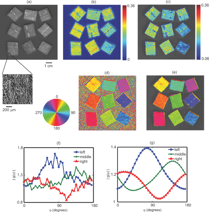

4.

Results

Figure 4 demonstrates the ability of SFDI to image the orientation of scattering structures at the surface of a turbid medium. Nine fiber samples from a pleated air filter were fixed at various orientations on the surface of an isotropic tissue simulating phantom and imaged as described above. A black and white photograph [Fig. 4a] shows the position of the fibrous samples. The inset is a confocal reflectance image of one of the fibrous samples in which the orientation of the microscopic fibers is visible. The SOI image [Fig. 4b] clearly indicates that the scattering from the fiber samples is more anisotropic than that of the surrounding medium. We then used an arbitrary threshold to aid in the display of the SOI. In Fig. 4c, only values of the SOI above the threshold value indicated on the color bar appear, and these values are superimposed over the black and white photograph. Figure 4d is a color coded image of the orientation of the microscopic fibers composed of the fibrous samples. The color wheel to the left gives the correspondence between each color and the direction it denotes. Starting from the bottom left and moving upwards column by column, the orientation of the fibrous samples is rotated clockwise. This is clearly shown in the image by the overall color of each fibrous sample. The areas between the fiber samples also are assigned values. This occurs because the processing code simply picks the projection angle for which each pixel has its minimum value. As expected, in areas where the scattering is isotropic, the assigned values are random. This motivates using the threshold from the SOI image to choose which pixels to display in the orientation image. In Fig. 4e, only pixels in which the contrast was above its threshold value are shown superimposed over the black and white image. For these pixels, the direction of the underlying structures was clearly measured. In Fig. 4f we plot the amplitude as a function of the projection angle for three individual CCD pixels taken from the centers of the fibrous samples in the bottom row. The plots in Fig. 4g are for the same three CCD pixels after the spatial and angular filtering described in Sec. 3.2. Each pixel is assigned an angle corresponding to the minimum of its curve.

A potential advantage of using SFDI to image scattering orientation, as opposed to methods involving polarization, is that diffuse optical methods such as SFDI use multiply scattered light. Thus, they are able to probe underneath the tissue surface at depths where light loses its polarization. In order to test the ability of SFDI to image subsurface scattering orientation, we placed thin sheets of highly scattering material (μ^′ _s = 1.5 mm⁻¹) over the fibrous samples. In Figs. 5a, 5b, we show images of SOI and fiber orientation, as the thickness of the overlying medium is increased from 0 to 600 μm. As the thickness increases, the SOI becomes smaller, and the image quality deteriorates. Nonetheless, even at a depth of 600 μm, the method assigns the correct orientation to much of the image. We quantified the degradation of image quality with depth by picking a 50 × 50 pixel (11.5 × 11.5 mm) region of interest at the center of each fibrous sample and calculating the standard deviation of angular values measured for each depth within the region of interest. We obtained standard deviations of 3.8, 4.7, 12, and 33 deg for depths of 0, 200, 400, and 600 μm, respectively. We also attempted to image through a silicon sheet with a thickness of 1 mm. At this depth no scattering orientation was detected. While it may be possible to penetrate more deeply using lower spatial frequencies and/or longer wavelengths, it is clear from Fig. 2 that lower frequencies come with the price of decreased sensitivity to the scattering orientation.

Fig. 5

Images of the (a) SOI and (b) structure orientation from an experiment in which a layer of highly scattering material was put on top of the fibrous samples. The top layer was varied in thickness from 0 to 600 μm.

Finally we evaluated the ability of SFDI to image scattering orientation in ex vivo samples of muscle (in this case chicken breast) and brain. As shown in Fig. 6a, four slices of chicken breast were positioned over the tissue simulating phantom such that the orientation of their muscle fibers was varied in 45 deg increments. The chicken breast clearly exhibited scattering anisotropy, and the imaged orientation matched our expectations, albeit with some biological variation. Figure 6b displays the results from imaging coronal slices of the brain of a rat. White matter composing the corpus callosum is visible in the black and white image. We expect that the oriented myelinated axons predominately found in white matter, will result in anisotropic diffusion of diffuse light. The myelinated axons are already known to cause the anisotropy diffusion of water, and form the basis for diffusion tensor magnetic resonance imaging (DT-MRI).³³ In the contrast image, areas of high contrast tend to correspond to white matter. Although we are unable to validate that the axon directions are correctly determined in this preliminary experiment, the orientation of white matter structures found with SFDI could be compared with DT-MRI in future work. These ex vivo experiments demonstrate the potential for using SFDI as a tool to image scattering orientation in biological tissues.

Fig. 6

Images of ex vivo samples of (a) chicken breast and (b) rat brain. From left to right: a black and white photograph, a SOI image, and a structure orientation image are shown for each sample. SOI and orientation images are superimposed over the black and white photograph after a threshold was applied.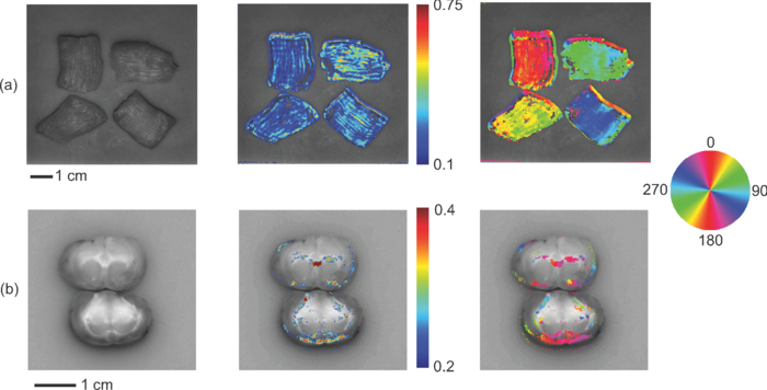

5.

Discussion

In this work we use a model of light propagation based on the diffusion approximation to the RTE. This approximation is known to be most accurate when 1. the reduced scattering coefficient is much larger than the absorption coefficient, 2. the distance between sources and detectors is much greater than one over the reduced scattering coefficient, and 3. the volume of interest is far from boundaries compared to one over the reduced scattering coefficient. In our experiment, conditions 2 and 3 are not met since the spatially distributed source is co-localized with all of the detectors, and we are only sensitive to anisotropy within ∼1 mm from the surface. Nonetheless, we (and others) have shown that the diffuse approximation can be used to accurately predict the diffuse reflectance from isotropic media.³⁴ However, we have also shown a slight increase in accuracy in our SFDI measurements of isotropic media when modeling light transport with Monte Carlo solutions to the RTE as opposed to using the diffusion approximation.¹⁴ We do expect the same qualitative results for SFDI using the anisotropic diffusion approximation as we would obtain by solving the full RTE. However, the extent to which the diffusion approximation can be used to model light propagation in anisotropic turbid media has been controversial,^{9, 35} and will be the subject of further SFDI research.

In this manuscript, we did not fit for the exact optical properties of the medium. Instead we determined the orientation and degree of anisotropy by finding the angle corresponding to the minimum measured amplitude, and defining a contrast function. Indeed, the anisotropic diffusion model contains many free parameters, and we have yet to determine to what extent we can solve for them using SFDI measurements.

Finally, it is important to point out that although we are using SFDI to image heterogeneous media, our solution to the anisotropic diffusion equation assumed the media was homogeneous. We analyzed the data from each CCD pixel independently assuming that the optical properties of the sample were sufficiently homogeneous such that the optical properties of neighboring locations did not affect the properties assigned to a given location. This was sufficient for demonstrating our sensitivity to scattering orientation, and for determining the orientation of the light scattering structures in two-dimensions. However, this approach has limitations. For example, the results of Fig. 5 clearly show that the measured contrast is determined not only by the properties of the fiber sample, but also by its depth. Thus, more sophisticated approaches involving layered models and/or tomographic imaging may be useful to facilitate quantitative measurements of scattering orientation in heterogeneous tissues. We have implemented both layered models¹⁹ and tomographic imaging²¹ for SFDI in isotropic media, and we expect to be able to extend these approaches to anisotropic tissues.

6.

Conclusion

We used SFDI to image the orientation of light scattering structures in highly scattering media. This was accomplished by rotating the orientation of sinusoidal patterns of light intensity projected on the sample, and measuring the attenuation in amplitude of the patterns as a function of the projection angle. We derived an analytic solution in the Fourier domain to the anisotropic diffusion equation, and defined a contrast function, the scattering orientation index, which gives a measure of the degree to which multiple light scattering has a preferred direction. We validated our approach by imaging tissue simulating phantoms as well as ex vivo samples of muscle and brain. We were able to distinguish between regions with isotropic and directional scattering, image the orientation of scattering structures embedded at a depth of 600 μm in highly scattering isotropic media (μ^′ _s = 1.5 mm⁻¹), and determine the scattering orientation within a standard deviation of 3.8 deg using individual CCD pixels. This technique may aid in the diagnosis of tissues such as skin, muscle, bone, and brain; in which the loss of orientated structure may be associated with disease.