1.

Introduction

In biological microscopy it is of great interest to investigate new methods for the automatization of intensive and repetitive tasks that requires a high degree of attention from the specialist. Slide scanning automatization procedures, from image acquisition to analysis, will be of benefit to the clinician from different aspects. First, by reducing the contact with the samples it is possible to realize a better analysis by minimizing alterations in the results and other risks. Second, this procedure will allow an increase in the number of fields of view to be analyzed, which is always a tedious task. In fact, an automatic system will provide more accurate diagnostics while reducing the time required for that purpose.

Although focusing can be a trivial task for a trained observer, automatic systems fail to find the best focused image from a stack under different modalities such as bright field microscopy (BFM) or phase contrast microscopy (PCM). Many autofocus algorithms have been proposed in the literature, but their accuracy can deviate depending on content of the processed images. Among the publications, a wide variety of autofocus methods have been evaluated. Osibote et al.¹ who determined that the method Vollath-4² had the best focus accuracy for bright-field images of tuberculosis bacilli. Santos et al.³ came to the same conclusion. However, other studies such as Kimura et al.⁴ and Liu et al.⁵ found the variance of pixels intensity as the most accurate method for tuberculosis and other blood smears. Furthermore, the study performed by Liu included additional assessment features like dynamic screening, shape of focus curve, or computation time which complicate the election of a unique method.

For a specific application, the election of a particular autofocus method will depend on two main aspects: the accuracy error and the computation time (see Redondo et al.⁶ for some preliminary results). Both criteria are important, but other features such as the number of local maxima, width of the focus curve or noise/illumination robustness can play a crucial role in automatic slide screening. Since the type of image on hand can determine which algorithm should be finally used, we evaluate in this paper a set of sixteen autofocus techniques considering the previous features specific to histological and histopathological images:biopsy, citology, autopsy, and tissue microarray. The paper is structured as follows. The employed materials, equipment, and the image dataset are described in Sec. 2. Section 3 describes the focus measures used in the present study and provides their mathematical foundations. Section 4 makes a comparative study of the experimental results. Finally, some conclusions and directions of future work are drawn in the last section.

2.

Materials

Specimens fixed in 4% buffered formalin were selected to prepare 3 to 15 μm thickness, histological slides deparaffinized in xylene. Thickness depends on the area and the histopathological test performed. Both conventional haematoxylin-eosin stain (HE) and immunohistochemical (IHQ) techniques were performed. Immunohistochemical detection on areas of paraffin embedded prostate, breast biopsies, and brain autopsies was performed using monoclonal mouse anti-human Ki-67 antigen (clone MIB-1, DAKO, Denmark), and polyclonal rabbit anti-human antibodies for Prostate-Specific Antigen(PSA, DAKO, Denmark). The immunocytochemical detection in cytology from pleural effusions was performed using monoclonal mouse antihuman calretinin (clone DAK-Calret 1, DAKO, Denmark), and papanicolau stain. In all tissue cases, target retrieval was performed with a pre-treatment module for tissue specimens, PT Link, (DAKO, Denmark). Ready to use primary antibodies were incubated for one hour at room temperature. The detection was performed using the EnVision $\mathrm{FLEX}+$ (DAKO, Denmark) visualization system in an Autostainer Link 48 (DAKO, Denmark).

The image stacks were captured from three lung cytologies with papanicolau and calretinin stain, the latter being a weaker staining. Lung cytologies were mainly liquid acquired with fine-needle aspiration, and they are the thinnest case among the studied cases. From these samples a blood area was considered in order to validate focusing robustness on delicate cases. Other analyzed samples were one prostate biopsy, one brain autopsy and one breast tissue microarray (TMA), whose density is similar to biopsy. In order to evaluate other realistic conditions, an additional breast TMA sample with air bubbles produced during the preparation was also tested.

Tissue samples were digitalized with a motorized microscope (Leica DM-6000B) controlled by using our own software developed by VISILAB research group. Images were $1392\times 1040$ in size and 8 bits of dynamic range in grayscale. An expert trained in pathological diagnosis task selected the best focal plane from which 20 images were captured upward in axial direction and another 20 downward, thus the stacks are made of 41 images where $Z$-step was 1 μm. Four different magnifications were used: $\times 10$ ($\mathrm{NA}=0.30$), $\times 20$ ($\mathrm{NA}=0.50$), $\times 40$ ($\mathrm{NA}=0.75$), and $\times 63$ ($\mathrm{NA}=0.90$). Significant differences in NA were tested to see how the optical contrast could affect the focusing metrics. Three stacks were captured with four different magnifications each from seven different tissue samples (papanicolau and calretinin lung cytologies, blood, prostate biopsy, brain autopsy, breast TMA, and TMA with air bubbles). The result was 84 stacks in total. See Fig. 1 for some examples. The best focus was finally obtained from an averaged evaluation from five experts. All algorithms were written in Matlab R2010 and run on Intel Core i7 Extreme Quad 3.07 Ghz, 4 GB RAM, HD SSD $6\mathrm{Gb}/\mathrm{s}$.

Fig. 1

Examples of microscopy images of size $1392\times 1040$. (a) Brain autopsy with magnification $\times 20$, (b) prostate biopsy $\times 40$, (c) calretinin lung cytology $\times 10$, (d) papanicolau lung cytology $\times 20$, (e) blood $\times 20$, (f) breast TMA $\times 63$, and (g) TMA with air bubbles 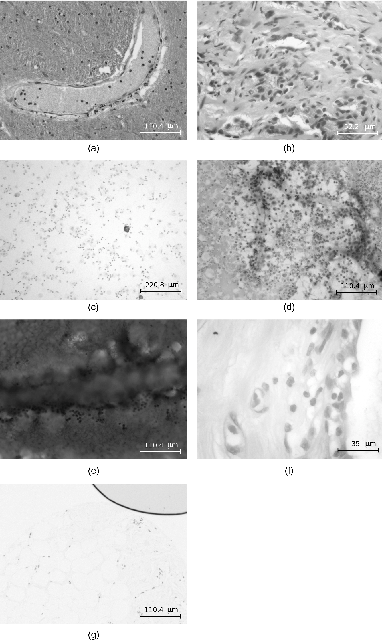$\times 10$.*

3.

Autofocus Methods

Autofocus is a property of an automatic system (e. g., microscope or camera that provides the optimum focus for specific objects in a scene). In the case of a camera, most of the autofocusing methods are based on external means by emitting ultrasonic or infrared waves. These methods are called active methods due to the way of measuring the distance between the lens and the object of the scene. Passive autofocus systems are based on analyzing the image sharpness of the objects, which is usually associated with a higher frequency content. In microscopy, the focusing procedure is carried out mechanically and is obtained by varying the distance between the objective lens and the subject of interest. In order to speed up the acquisition process in automated microscopy, the search for the best focus cannot be extended to a whole number of stacks in real-time applications. A good slide screening strategy could be to first perform a coarse search of large steps guided by a simple focus measure with low computation time and then switch to a finer search where a significant difference between two consecutive image captures appears.⁷ Automatic systems often fails to focus images under different microscopic modalities. Therefore, a desirable focus measure should be evaluated in terms of reliability, accuracy, and speed. Most of the methods proposed in the literature can be classified into five groups: derivative, transform, statistical, histogram, and intuitive-based methods.⁸

In this study, a wide set of focus measures from the already well known methods to those proposed recently have been analyzed. Some of these measures have been specifically proposed for autofocusing bacteria specimens,^9,10 while others have not been tested within this particular context.¹¹ Other focus measures, such as⁴ Brenner gradient and entropy method,³ have not been included here, but they belong to the same family of Vollath and histogram techniques. In the next lines we summarize the main characteristics of the focus measures selected for the current study. For an image of size $M\times N$, the notation $g$($m$,$n$) refers to the image intensity at point ($m$, $n$), while the symbol * indicates the convolution operator.

Fig. 2

Main diagonal coefficients corresponding to a $8\times 8$ pixels block. In our case, the image is divided into blocks of $40\times 40$ pixels to reduce the computation time.

We also experimented with Hu moments^21,22 but the results were not included here due to their low performance in this framework. Since the time-to-focus calculation could vary depending on the implementation of each algorithm, the Matlab code can be downloaded from http://www.iv.optica.csic.es/page49/styled/page59.html.

4.

Experiments

4.1.

Accuracy Error and Computational Cost

The error of the algorithms applied to the seven types of stacks is depicted in Fig. 3(a). The abbreviations GS1, GS2, and GS03 are related with the Gaussian method for respective sigma values of $\sigma 0.1$, $\sigma =1$, and $\sigma =10$. Furthermore, the lines drawn above the bars indicate the variance of data. According to such plots, most of the algorithms show high performance (between 2 and 4 μm which indicates a 2 to 4 frame distance) except TH and DCT. TH manifests strong dependency on selecting an appropriate threshold and has difficulties at high magnification factor [see Fig. 3(b)]. The lowest mean error corresponds to ATEN of 2.65 μm. Although it is not presented here, the lowest error is achieved for weak-stained cytologies, below 1 μm for most methods. In contrast, the error is triggered for the TMA with bubbles up to 10 μm for most of the methods. Figure 3(b) presents the mean error for separate magnification factors, or NA. With the exception of the TH method, one can see that all the algorithms drastically impair their accuracy at $\times 63$ factor, and others like DCT method impairs even at $\times 40$ [see Fig. 3(b)]. This is consistent with the fact that higher magnification objectives provide a shallow depth of field. Such reduction could be mitigated by increasing the size of the DCT kernel at the expense of simultaneously increasing the computation time.

Fig. 3

(a) Global error performed by the autofocus measures and (b) global error according to the magnification value (NA) (right).

For real-time applications, a trade-off between computational cost and accuracy is necessary. Thus, the algorithms with the best ranking in terms of computational cost are not necessarily effective in terms of accuracy (see Fig. 4). We considered more realistic to provide a relative comparison among all the methods rather than taking an absolute measure. Notice that in a real system implementation using a compiled language such as C or C++, or even if we consider an embedded architecture, the absolute values would vary significantly. From the evaluated algorithms, the TH method was the fastest with 2.5 ms per image. Hence the computational time employed for this algorithm was taken as a reference for comparing the time of the other measures. Based on these results, the measures with the lowest error performance but also fast implementation are VAR and NVAR, followed by VOL5 and MDCT. These algorithms where also tested on a Mac mini Intel Core Duo 2.4 GHz, and we discovered some fluctuations for DCT, but the rest of the methods behaved quite stable.

Fig. 4

Averaged computation time factor compared to the fastest algorithm TH (scored $\times 1$).

4.2.

Noise and Non-Homogeneous Illumination

The performance of autofocus measures have been evaluated when noise and illumination changes are added to the stacks. In the case of noise, we have added increasing levels of zero mean Gaussian noise to the original data and calculated their influence in the accuracy error. Although the used values are far from the normal usage conditions, this experiment can provid extra information about the true robustness of the focus functions. The results for noise robustness are summarized in Fig. 5. Notice that most of the methods are reasonably stable until the distortion becomes extremely large, with the exception of DCT, MDCT, LAP, and TH which manifest more sensibility to noise. GS, PS, VAR, and VOL5 are among the most robust.

Fig. 5

Reponses of the focus functions to (a) zero mean Gaussian noise and (b) center-radial illumination.

The non-homogeneous illumination was simulated using a radial luminance pattern, [see Fig. 5(b)] whose representation as a gray-level image was added to the original images and normalized to the maximum gray-level of the original image. For this test, different intensity maxima were used which can be observed in the small pictures inside the plot. The focus measure TH is highly sensitive to this type of distortion which could be mitigated by the election of an optimum threshold. However, in any case, this evidences its lack of robustness. Power squared focus measure is highly dependent on the illumination, probably because it relies on overall power of the image contents.

4.3.

Accuracy in Focus Curve

A key aspect in the automatization process is to determine reliable and fast autofocusing methods. In such automatization processes the shape of the focus curve can play an influential role. Groen et al.¹⁴ used eight different criteria for the evaluation of autofocus functions. Figure 6 stands for a schematic representation of the main characteristics of an autofocus curve. Ideally the focus function should be unimodal, but in practice it can present various local maxima which can affect the convergence of the autofocus procedure. Moreover, the focus curve should ideally be sharp at the top and long tailed, which can accelerate the convergence of the screening procedure when the whole slice is scanned. This way, in order to have a more complete characterization of the autofocus algorithms, we have verified the shape of their autofocus curve by taking into account two aspects: the number of local maxima and the width ratio, expressed as: $\text{width}=\alpha /\beta$, where $\alpha$ and $\beta$ are, respectively, the width of the focus curve at 80% and 40%.

Fig. 6

Autofocus curve characterization by the number of local maxima $\eta$ and the width ratio at 80% and 40% of the maximum $\text{width}=\alpha /\beta$.

First, one can observe in Fig. 7(a) that most algorithms present a unique maximum as averaged value, except LAP, PS, TH, VOL4, TEN, and ATEN, and the worst cases are DCT and MDCT. With respect to the width ratio of the focus curve, (see Fig. 7(b)) no significant discrepancies are found. In Table 1 summarizes some of the most accurate and/or the fastest algorithms, where VAR, NVAR, and VOL5 show high performance for the three aspects.

Table 1

Comparison of the most accurate and/or fastest algorithms.

	Mean error (μm)	Comp. time ($\times 1$)	Local Max.
GS03	3.5	15.92	1.13
TH	9.76	1.00	2.26
VAR	3.66	3.02	1.01
NVAR	3.63	3.19	1.07
VOL4	3.34	11.12	1.83
VOL5	3.65	6.38	1.01
TEN	3.63	14.13	1.77
ATEN	2.65	14.62	1.79
MDCT	3.63	6.97	5.08

Fig. 7

Comparison of focus measures in terms of (a) averaged number of local maxima (included the global maximum) and (b) averaged width ratio of the focus curves.

5.

Conclusions

In biological microscopy it is of great interest to investigate new methods for automatizing laborious tasks that require a high degree of attention from the specialist. Therefore, slide scanning automatization procedures, from image acquisition to analysis, will be of benefit to the clinician. We have presented here a study of focus measures to automate the acquisition of histological and histopathological images.

According to the results, most of the methods exhibit a low accuracy error, but only NVAR, VAR, and VOL5 simultaneously exhibit a faster implementation and a low number of local maxima. They could be considered as suitable candidates for an automatic system. Moreover, considering external distortions such as noise and non-homogeneous illumination, the last two candidates perform more robustly. If the computational efficiency is even more exigent, an alternative solution could consist of applying the fastest algorithm as a coarse search, that is TH, and then performing a finer search with another fast and accurate algorithm.

Future work is required for defining efficient whole slide scanning strategies such as using a coarse to fine search procedure or other optimal search methods. Even further, the use of Field Programmable Gate Arrays (FPGAs) or the General-Purpose computation on Graphics Processing Units (GPGPU) will be considered in the future for increasing the overall performance of an autofocus system. The FPGAs parallel processing and high speed capability will speed up both the image processing and focusing control parts that are limiting factors in an automatic acquisition system. In particular, the implementation of the better performant autofocusing methods in FPGA architectures will allow the parallel execution of them and therefore to select the most accurate method almost in real time. The selection procedure can be implemented e.g., through an evolutionary algorithm. Another fast but less accurate algorithm could be included to cope for pre-screening tasks. Finally, it is necessary to remark that this type of technique will come to help the clinician specially in those repetitive and tedious tasks such as image acquisition and autofocus, but they do not replace the expert until image analysis methods become effective.