

|
|
1.IntroductionAcousto-optics (AO), or ultrasound-modulated optical tomography, is a hybrid technique which combines the optical contrast of biological tissues at visible or near-infrared wavelengths with the spatial resolution of focused ultrasound fields to provide highly localized measurements of the optical properties of biological tissues. Such measurements are of clinical significance since they may indicate underlying pathologies, e.g., increased vascularization due to tumor angiogenesis, or serve as an indicator of the progress of treatments which themselves alter the optical properties of tissues, e.g., thermal necrosis by therapeutic high-intensity focused ultrasound (HIFU).1 1.1.Acousto-Optic ModelingLeutz and Maret2 first developed a model of the AO effect in turbid media based upon the approach of diffusing wave spectroscopy (DWS)3,4 with the addition of sinusoidally oscillating optical scatterers. Kempe et al.5 extended the analysis of Leutz and Maret to consider a narrow beam of ultrasound and compared this model to experimental data. Mahan et al.6 proposed the acoustic tagging process to be that of Brillouin scattering, proceeding to develop an expression of the intensity of the modulated signal and the signal-to-noise ratio in the case of an ultrasound field focused into a small volume. Theoretical understanding of the technique was advanced by Wang,7 who jointly modeled the two coherent mechanisms of interaction previously investigated: the acoustically induced displacement of optical scatterers and the change in the index of refraction due to compression and rarefaction. Theoretical research continued with the extension of Wang’s model to the case of anisotropically scattering media8 and to account for strong correlations in the interaction at successive scattering sites.9 Blonigen et al.10 further investigated the nature of the phase shifts applied to ultrasound modulated light in the context of a photorefractive crystal detection regime. The inherent limitations of theory based upon the DWS approach were overcome by Sakadžić and Wang through the development of a correlation transfer equation (CTE)11 which provides a treatment of the acoustic continuous-wave (CW) AO problem in the style of a transport equation. A diffusion approximation (DA) is presented in a subsequent work,12 and later the CTE is reformulated to account for an ultrasonic pulse.13 Recently Bratchenia et al.14 developed sensitivity maps of the acousto-optic technique based upon a pair of coupled diffusion equations accounting for the unmodulated and modulated distributions of light. Throughout the initial theoretical investigations of the technique, a number of CPU-based Monte-Carlo (MC) models were demonstrated to support the analytical solutions under development.8,9,11–13,15 1.2.GPU-Accelerated Monte-Carlo TechniqueIn recent years, considerable advances have been made in executing MC simulations on the highly parallel architecture of graphics processing units (GPUs). The first demonstration by Allerstam et al.16 considered the problem of light transport in an homogeneous semi-infinite medium; increases in speed over a CPU implementation of up to three orders of magnitude were achieved. Fang and Boas17 subsequently developed a general purpose code to perform MC simulations in heterogeneous voxelized geometries. Under specific circumstances speed increases over a CPU implementation of up to were noted. We recently demonstrated the acceleration of a MC AO simulation,18 achieving performance improvements of up to over a CPU implementation equivalent to that presented in Ref. 15. We also demonstrated that our GPU-based AO simulations involved an order of magnitude of extra computational effort over a pure optical simulation. 1.3.AimsGiven the demonstrable improvements in efficiency which can be achieved using a GPU-based parallel implementation, our aim is the development of a robust, efficient and flexible simulation tool that has the potential to provide significant guidance in the application and optimization of the AO technique as both an imaging and a sensing modality for a broad range of tissue geometries and detection mechanisms. A fast forward model may also serve as the basis of future developments in inversion techniques for AO. While our previous implementation18 was limited to homogeneous semi-infinite slab geometries with plane-wave ultrasound, here we develop a code capable of simulating the AO effect in optically heterogeneous domains, with arbitrary (monochromatic) acoustic field distributions. Previous CPU-based simulations reported in the literature11,13 have implemented a similar level of flexibility by the use of a voxelized simulation domain for the spatial distribution of the optical and acoustic parameters. Here we will demonstrate the implementation of optical heterogeneity via a mesh-based system which avoids the deleterious effects of a voxelized geometry,19 and exploits the computational power of the GPU to avoid approximations in the treatment of the AO phase shifts demonstrated in previous work.11 It is our intention to release the described simulation code publicly in the near future; if you wish to be contacted upon its release, please contact the corresponding author by E-mail. 1.4.OverviewWe begin in Sec. 2 with an overview of the relevant theory of AO, and the variance-reduction technique employed for point-source, point-detector (PSPD) simulations. The implementation of the simulation program and its post processing techniques are detailed in Sec. 3, following a brief overview of the pertinent considerations of parallel programming for GPU architectures. In Sec. 4 we demonstrate the validation of the simulation program, consider its performance relative to other simulation codes, and demonstrate one application in the calculation of explicit spatial sensitivity maps corresponding to experimental studies currently being undertaken. This work closes in Sec. 5 with a discussion of the limitations and possibilities for future development of the simulation code. 2.Theory2.1.Acousto-Optic Interaction within Turbid MediaThree modes of AO interaction have been proposed in the literature: displacement of optical scatterers in a turbid medium by the acoustic field,2 perturbation of the refractive index of a medium due to mechanical strain induced by the acoustic field,7 and perturbation of the optical properties of the medium due to compression and rarefaction of the medium by the acoustic field.6 The latter mechanism could in principle be detected with incoherent light, but this effect has been too weak to be detected in practice (without the use of fluorescence). We consider only the two former mechanisms, which require the use of coherent light. 2.1.1.Variation of the index of refractionAn acoustic wave propagating through a medium generates a strain which alters the local permittivity of the medium. The adiabatic piezo-optic coefficient ( in water) relates the change in the index of refraction to the acoustic pressure .20 Consider a plane electromagnetic wave propagating between two points and with wavenumber , where is the angular frequency and the speed of light in vacuo. The incremental phase angle accrued on this path over that of an optically homogeneous medium of refractive index is given by Under insonification by a monochromatic acoustic field of angular frequency , local pressure amplitude , and local phase offset relative to an arbitrary point we express the complex time harmonic phase increment2.1.2.Displacement of optical scatterersAn acoustic wave propagating through a turbid medium displaces the endogenous optical scatterers from their rest positions. The acoustic particle displacement at an arbitrary point in space and time is where is the unit acoustic propagation direction derived from the acoustic wave-vector and wavenumber , is the density of the medium and the speed of sound in the medium. We express the complex valued acoustic particle displacement for a monochromatic acoustic field and assume that the displacement of a given scatterer follows that of the background medium with a particular phase offset and scaled amplitude ,10 Assuming two scattering sites at and are separated such that they are in the far-field zone of one another, the phase increment accrued by an electromagnetic wave will be the projection of the optical wavevector onto the overall scatterer displacement,2.1.3.Acousto-optic interaction in a multiple scattering regimeWe may think of the electric field at a point within, or on the boundary of a coherently illuminated turbid medium to consist of the summation of an unscattered field resulting from the incident radiation and numerous partial fields which result from the multiple scattering process, where denotes the unscattered field due to the incident radiation, and the partial multiply scattered fields, each representing a contribution from a scattering process of some order. Direct calculation of the electric field by this approach is impractical for any realistic biological system. Transport theory treats the multiple scattering problem by considering the propagation of wave-energy in directed rays (essentially the short wavelength limit of wave optics) traversing a medium according to statistical considerations of the underlying turbid media. The MC technique employed in our simulation ‘samples’ this interpretation by propagating a finite number of quasi-plane-wave rays of wave energy21 which sum together to approach the solution to the underlying transport equation. Our problem thus reduces to defining the manner in which these rays propagate, and their associated phase perturbations due to the acousto-optic interaction.Over sequential scattering events at , , the phase increment of Eq. (6) becomes a summation . With , we can write the phase increment upon incidence with a scatterer located at , where and represent the optical wavevectors prior to and following incidence with the scatterer, respectively. Thus, over a scattering path involving free paths and scattering events we may write the complex phase perturbation, where is a particular scattering event, is the input location, and is the location where the ray is detected. Taking the magnitude and phase angle of this perturbation we may express the time varying phase increment as10 Each of our quasi-plane-wave rays will thus take the form where is some amplitude, some random phase due to the multiple scattering process for this ray, the AO phase shift for this ray, and the optical frequency.2.2.Observables and MeasuresFollowing multiple scattering in a turbid medium, the field variable will be a random variable fluctuating over time as effects such as Brownian motion alter the contributions from its constituent scattering paths. Nonetheless, we may investigate the effects of the AO modulation by means of the temporal-field autocorrelation function, , which is derived from the observable temporal-intensity autocorrelation function, , by the Siegert relationship, In the context of our simulated quasi-plane-wave rays (herein photon packets), Neglecting Brownian motion (e.g., removing the time dependence of ) and under the assumption that the system is ergodic and wide-sense stationary, only those terms in the electric field which vary deterministically over time are retained in the expression for . Thus the integration can be performed by expansion of the exponentiated cosine via the Jacobi-Angers identity,22 where is the ’th Bessel function of the first kind. We recognize that the modulation index, , is proportional to the acoustic pressure amplitude [as demonstrated in Eqs. (2), (5), and (8)] and that the phase modulation expressed in Eq. (10) has caused the monochromatic optical input to be partially shifted in frequency. By the Wiener-Khinchin theorem the power spectrum of the detected field is given by the Fourier transform of the field autocorrelation function; this can be seen by inspection to consist of a DC component and numerous side-bands at multiples of the acoustic frequency, each scaled by a squared Bessel function of increasing order.2.3.An Adjoint Method for AOMC models of light transport are unable to directly simulate PSPD regimes which commonly occur in studies involving the use of coherent light, since the random walk process is unlikely ever to impinge directly upon the detection point. One approach to estimating the value of a quantity at a point with the MC method is the use of the adjoint method, as applied in the case of standard photon and neutron transport.23,24 We now expand this concept to the case of AO where energy will be distributed not only at the input optical frequency, but at sidebands shifted by multiples of the acoustic frequency. A pencil beam incident normal to the boundary of the simulation domain at some point illuminates the system with a given irradiance, . We denote the probability of optical power at some point in the ’th sideband reaching some point in the ’th side band as . The probability distribution of optical power at each sideband throughout the domain resulting from the source at is given by the unitless normalized fluence rate , where is the fluence rate at a point in the medium in the ’th side-band. In replacing our detector with an adjoint source of equivalent directivity at , we may derive another set of optical power probability distributions . The Chapman-Kolmogorov equation states25 In the case of transitions to and from different side bands we must sum over the relevant permutations: We assume that contributions to the ’th side-band are negligible and thus express the detected exitance at the zeroth side-band, where by optical reciprocity . The detected exitance at the first sideband is given by, We find by optical reciprocity, and make the approximation . Thus, the first side-band modulation depth [] detected at a point on the boundary is given by3.Implementation3.1.GPU Parallel Programming in the CUDA FrameworkThe design of an efficient GPU-accelerated parallel algorithm requires careful consideration of the underlying computational architecture. An extensive discussion of best practices is provided by the authors of the CUDA architecture.26 Our implementation follows three broad strategies.
3.2.ArchitectureThe simulation program is built around the light-propagation and phase-accrual algorithms of the propagation kernel. Many thousands of instances of the kernel each execute in parallel on the GPU, the configuration and execution of which is managed by the driver. The driver consists of a MATLAB frontend to the simulation executable. The user configures the simulation by building a set of MATLAB variables and structures with the data required to define the simulation domain; this includes the geometry, medium properties, acoustic-field distribution and various simulation constants. The simulation is executed by passing this configuration structure to the MATLAB driver function. The driver validates the input data, constructs any dependent data, and calls the simulation executable. The executable uploads the data to the graphics card and repeatedly calls the kernel to propagate a certain number of photon packets until the desired number have been propagated. The output data is collected and stored in a MATLAB data file. The architecture of the simulation program is depicted in Fig. 1. Fig. 1Architecture of the simulation program illustrating the parallel execution of many thousands of individual propagation kernels, each responsible for a single photon packet. 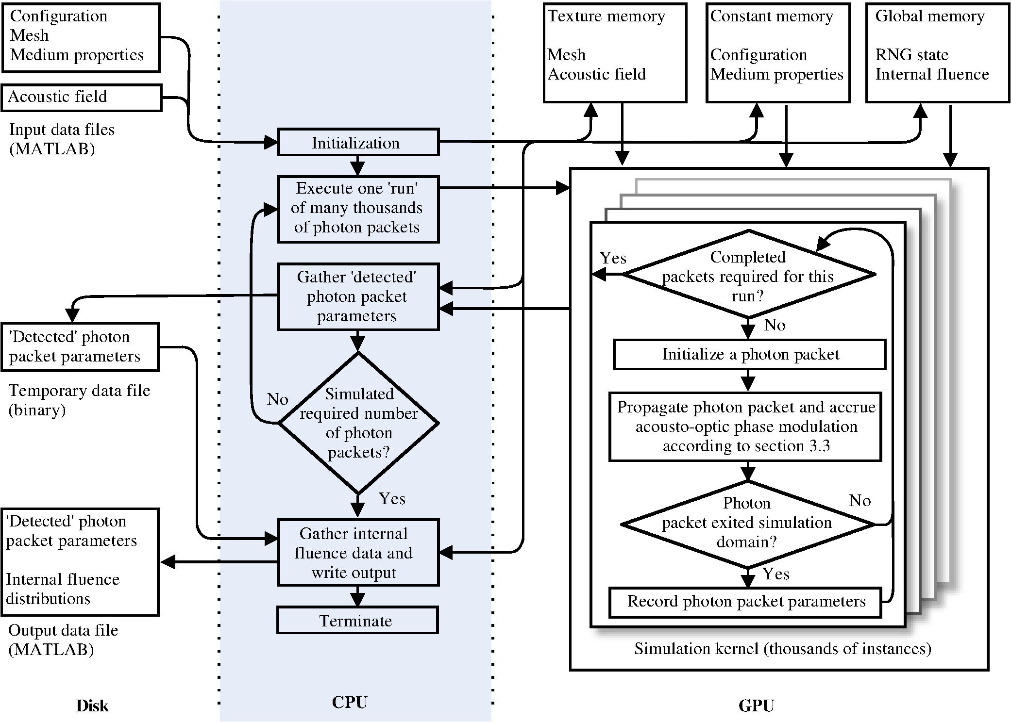 3.2.1.GeometryMany MC simulation programs which support heterogeneous optical properties, including GPU-accelerated programs17 and those which consider AO,12 implement heterogeneity by discretizing the domain into a voxelized grid. As a photon packet takes a step through multiple volume elements (voxels), each must be examined to ascertain if there has been a change in optical properties. While this approach has the benefit of being conceptually straightforward, representations of complex curved features require a very fine voxelization. Even with a fine voxelization, many of the problems discussed in Ref. 19 cannot be overcome. A different approach is taken here whereby the simulation domain is represented by a tetrahedral mesh. This representation is typically encountered in applications of, e.g., the finite element method, but has also been applied to a CPU-based MC photon propagation problem.27 By employing this method, photons move around within tetrahedral volume elements which subdivide the simulation geometry. On each photon step, we must check for intersection with any of the four facets of the current element; whilst we must still interrogate a dataset to determine the location of these facets, the amount of data to be retrieved, and the nature of the processing to be performed, is now fixed across each thread, thus avoiding issues of divergence and potentially reducing the amount of data which must be retrieved from memory relative to a voxelized solution (dependent upon the complexity of the model). Many of the advantages of this approach are discussed in Ref. 28. The meshed geometry is represented by four sets of data. The first is the node list, which records the three-dimensional (3-D) Cartesian co-ordinate of every node, or vertex, in the mesh. The node list is used by the element connectivity matrix, which defines individual tetrahedral elements by indexing four such nodes. In addition to this data, we also provide a list of element neighbors that for each element provides an index into the four neighboring elements. Finally, the properties table indicates the medium of which an element is composed by providing an index into the medium array. Each of the geometry tables is stored on the device in texture memory, which, whilst residing in the slow global memory, is spatially cached. This will convey significant advantages at the start of simulations when all photon packets reside in the same element. 3.2.2.Geometry intersectionThe intersection of a line segment with a triangle is a well understood geometric operation. The most basic form of this test involves testing for intersection of the line with the plane defined by the three points of the triangle; many fast algorithms are available in the literature, one of the more popular being that of Möller and Trumbore.29 When such tests are implemented with finite precision, errors in the intersection tests may occur; this can often be tolerated in graphics rendering, for which such ray-tracing algorithms are typically developed. In this application the consequences of such an error is that a photon packet will end an iteration of the algorithm at a position which does not correspond to its current element; all subsequent intersection tests will fail and the photon will propagate indefinitely, or be fully absorbed within an incorrect element. This problem is exacerbated by the use of single-precision floating-point arithmetic within the kernel (the most efficient data type for current GPU architectures) rather than the double precision typically employed in a CPU-based algorithm. A more robust approach is based upon the triple scalar product. In this case the majority of the tests are based upon the sign, rather than on the absolute value of the arithmetic operations. This approach is mathematically equivalent to the use of Plücker coordinates (as described by Fang27), but avoids the associated complexity of analysis and notation. The signed volume of a tetrahedron defined by four vertices is calculated by30 where is the dot-product and the cross-product operator. To determine if the ray defined by the current photon direction intersects the current tetrahedral element, we begin by retrieving the four vertices of the element from the geometry cache. We test for intersection with each of the four facets of the tetrahedron by iterating over the four choices of the three nodes. We ignore the result of a test against the facet, if any, over which the photon packet previously reflected or refracted.For each of the four facets we calculate three signed volumes , , and . In the case that the sign of each of these volumes is equal, the ray intersects the tetrahedron. To determine if the photon packet will intersect the tetrahedron given its current step size, we calculate the two signed volumes and ; in the case that the signs of these volumes are opposite, and that , intersection occurs at the parametric distance . If any interactions occur, the smallest intersection distance is used to scale the current photon step size. 3.2.3.Acoustic fieldAs discussed in the theory, simulation of the AO modulation process requires knowledge of the local acoustic pressure amplitude, , the local acoustic wave-vector, , and the local acoustic phase offset relative to some point, . We pack this data into a four-element array by storing, for each point, , where is the component of the normalized wavevector. The magnitude of is stored in constant memory to permit recovery of the wave-vector when required. We store the acoustic field data in a 3-D texture to exploit hardware caching, hardware-based trilinear interpolation (interpolation of the acoustic-field dataset is only possible when the phase angle of the field is unwrapped; if discontinuities around exist, interpolation will produce undesired effects), and normalized addressing. It is thus possible to read all needed parameters of the acoustic field at a given location in one texture access. 3.2.4.MediumEach medium is represented by a structure stored in constant memory containing the absorption coefficient, , the scattering coefficient, , the anisotropy factor, , the index of refraction, , the piezo-optic coefficient, , and the speed of sound, . 3.2.5.Random number generatorOn numerous occasions within the light-transport algorithm a uniformly distributed random number must be generated. This application uses an implementation by Alerstam16 of Marsaglia’s multiply-with-carry random number generator.31 As described in the references, the algorithm requires only eight bytes of state information and has a period of greater than . 3.3.The Monte-Carlo ProcedureMany of the fundamental calculations performed are of a standard form for MC light-transport codes; Wang’s description32 of his de facto standard code, MCML, will serve as a reference for these processes. We implement the following general procedure for light transport:
4.Results4.1.ValidationThe optical model of the simulation code has been validated against numerous analytical formulations based upon the DA to the radiative transfer equation (RTE). Simulations have been performed to compare the code to the total diffuse transmittance and total reflectance of van de Hulst,34 the total reflectance as calculated in the multi layer diffusion model of Liemert and Kienle,35 the temporal point-spread functions (TPSFs) presented by Martelli et al.,36 and the internal fluence for an optically inhomogeneous sphere inside a semi-infinite slab as derived by Boas et al.37 In each case, excellent agreement is found in regions where the DA is valid. The optical model has also been compared against the output of MCML.32 A variety of simulations were performed in optically heterogeneous multi layered geometries. In all cases, excellent agreement was found in the total diffuse transmittance, total reflectance, and the radially resolved output. Fewer analytical formulations are available with which to validate the AO model. Sakadžić and Wang8 present a set of figures [Figs. 2(a)–2(d)] demonstrating the as derived by the analytical solution for AO in a slab geometry with plane-wave ultrasound. These figures have been recreated and demonstrate excellent agreement over each demonstrated permutation of the acoustic and optical set up. In subsequent work Sakadžić and Wang12 employ their correlation diffusion equation to calculate the within a highly scattering, optically homogeneous semi-infinite slab of width , insonified by a cylinder of plane-wave ultrasound. Fig. 2[] evaluated along the reflection (, lower curve) and transmission (, upper curve) surfaces of the slab in the plane of the source as calculated by the simulation program and the correlation diffusion equation. Excellent agreement is seen with the diffusion equation away from the source location in the reflection surface (, ).  We recreate this simulation by generating a cuboid mesh of width . The depth and height of the mesh (, ) are chosen to minimize boundary effects. A cylinder of ultrasound is created of radius 3.175 mm. Ten million photon packets were launched into the domain at , and allowed to propagate until they were completely absorbed into the medium or exited the domain via one of the boundaries. The simulation program recorded the internal fluence distribution on each node throughout the medium at the input optical frequency, , and at the first shifted side band, . The internal first side-band modulation depth was calculated as prior to interpolation to a regular grid using standard MATLAB functions. Figure 3 plots the internal first-side band-modulation depth inside the slab in the plane of the source. Figure 2 compares the MC simulation against that of the analytical solution along the transmission and reflection planes of the slab. Excellent agreement is found over the region where the DA is valid. Near to the source location we note a large dip in the , as would be expected when the large unmodulated intensity is considered. The MC results agree excellently with those presented in the original work.12 Fig. 3[] for a cut through the slab in the plane of the source. The source is incident normal to the slab surface at , . The column of ultrasound is centerd at , , as indicated by the white circle. 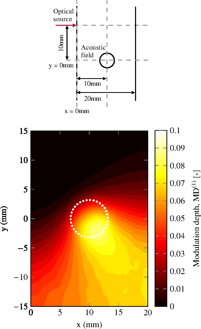 In each of the simulations performed for the validation procedure, the explicit acoustic integration technique was employed since this is exact in the case of plane-wave insonification. Use of the numerical integration method with six points per wavelength produced identical results for this particular set of acoustic and optical properties. 4.2.PerformanceTo illustrate the performance of the simulation code, we compare its optical performance against a recent CPU mesh-based MC model, MMCM.27 We execute the simulation of the inhomogeneous sphere in a scattering slab using the same mesh (MMCM Mesh 2) as used by Fang,27 who reports a speed of 5.6 photon packets per millisecond () for a single thread, scaling to when executed over four threads. Our GPU implementation processes while executing on a single nVidia GTX 250 graphics card. The GPU implementation executes at almost eight times the speed of the single core CPU implementation, or almost twice that of the four-core parallel implementation of Fang.27 The GPU implementation may be executed on a server incorporating multiple GPUs, where performance will scale linearly according to the number of devices available. While calculation of the AO phase shifts was disabled at run time, the overhead of variable definitions at compile time still has considerable performance implications owing to the number of threads which may execute simultaneously. Removal of the AO aspects of the simulation code should be expected to significantly improve performance if only an optical simulation is required. Very little data has been published with which to compare the performance of the code in the AO case. We recently presented the results of a GPU-based slab geometry plane-wave AO code and compared these to a CPU implementation18 of the same. We now compare the performance of the current simulation code to that of both the CPU and GPU codes demonstrated previously. A semi-infinite slab of depth 2 cm (represented in the current simulation code as a slab of lateral extent 10 cm) with optical properties , , , and varying is illuminated on one surface and the AO determined given insonification by a plane-wave acoustic field of displacement amplitude and varying frequency. Table 1 details the speed of the simulations in numbers of photon packets per millisecond. The previously reported simulation figures are given in the column labeled GPU Orig., the speed of the current simulation is described for two frequencies and for both the numerical integration of phase of Eq. (20), and the explicit integration of Eq. (22). Table 1Execution speed (photon packets/ms) of alternative acousto-optic simulation programs and configurations. Numbers in parentheses demonstrate the speed-up relative to the CPU implementation.
To understand the resultant performance data, we must consider the limiting factors in each of the simulation algorithms. The performance of the original CPU and GPU codes is primarily a function of the scattering coefficient, , since this dictates the number of calculations which will be performed for a given photon packet’s simulation (as discussed further in our earlier work18). The new simulation code retains the same performance dependency while introducing two further factors which may affect performance.
The aforementioned qualities of the performance of the new simulation code are evident in the performance data of Table 1. Under insonification by ultrasound at a frequency of 1 MHz (when the acoustic wavelength is long compared to a mean free path) geometry intersection tests (and their associated memory access) dominate the execution time and the new simulation code performs similarly under both integration regimes. The increased flexibility and associated complexity of the new simulation decrease the performance of the new code relative to the previously reported GPU implementation. The new code achieves a performance varying between th and th of the previously reported GPU code; as increases, the speeds of the two GPU codes approach one another, since fewer geometrical intersection tests are processed in the new code relative to the total computational workload. Under 10 MHz insonification the explicit integration mode of the simulation maintains similar execution speed to that of 1 MHz insonification, though the numerical integration shows a significant relative degradation in performance at low values of . In all but one of the examples investigated here the new simulation code is at least an order of magnitude faster than the CPU implementation; though as discussed, performance could be degraded by introducing a finer mesh, or in the case of the numerical integration mode, a higher frequency of insonification. 4.3.Sensitivity MappingIn recent work, Gunadi and Leung38 demonstrated the measurement of spatial sensitivity maps for the AO sensing technique. In this work an optical absorber of , , and dimensions was moved around a tank of intralipid of negligible absorption and equal scattering to that of the absorber. In the first case a transmission-mode geometry was investigated, with an optical source and detector separated by 35 mm. The absorber was moved around the central region in 1-mm steps over a grid, in each case the detected optical intensity (in the absence of ultrasound) and the AO (in the presence of ultrasound) were recorded. A reference measurement was taken in the absence of an absorber such that the sensitivity can be represented as , where may be optical intensity or AO , and is the corresponding reference measurement. We recreate this experiment in simulation though reduce the absorber size to a cube. The linear acoustic field is generated by distributing monopoles over the surface of a spherical cap of equal dimension to the transducer used in practice, and summing their contributions in the field. The amplitude is scaled to match that recorded by Gunadi and Leung.38 The mesh and absorptive inclusion is built on the fly using the iso2mesh toolbox. Following simulation, the adjoint method described in Sec. 2.3 is used to calculate the detected . Figure 4(a) and 4(b) depict the optical and AO spatial sensitivity recovered by 1250 independent MC simulations, each of two million photon packets. Fig. 4Spatial sensitivity maps (-% change from reference value). Inward arrows depict the source and outward arrows the detector location. The dotted ellipse illustrates the focus of the ultrasound region. (a) Transmission-mode optical sensitivity, (b) transmission-mode AO sensitivity, (c) reflection-mode optical sensitivity, and (d) reflection-mode AO sensitivity. 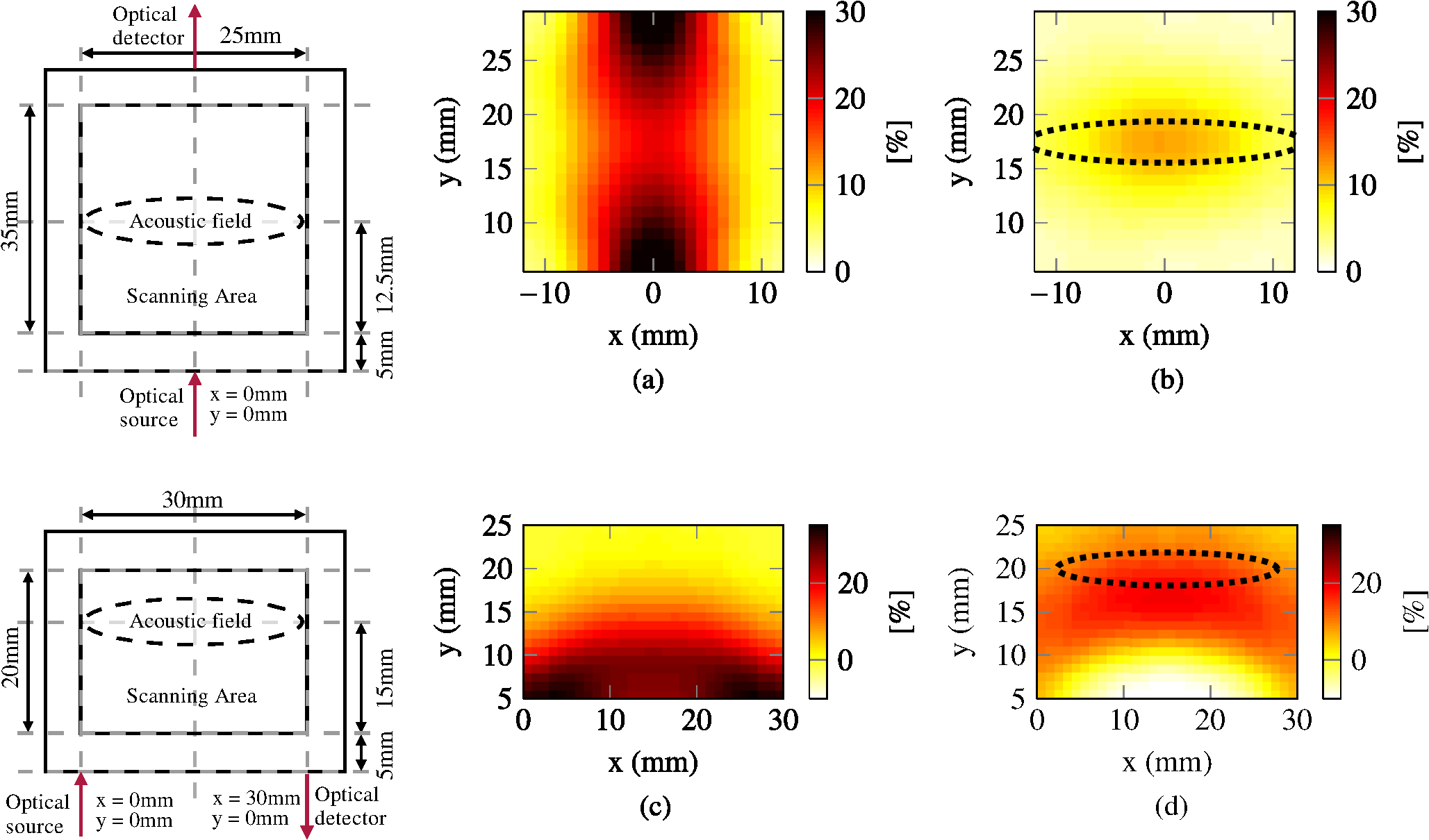 While the smaller absorptive inclusion leads to differences in the absolute sensitivity demonstrated by measurement and simulation, the form of the sensitivity distribution retains the same qualities as described by the experimental observations of Gunadi and Leung.38 As would be expected, the optical sensitivity remains concentrated around the source and detector locations. The AO sensitivity demonstrates localization to the acoustic field and, more significantly, a very low level of sensitivity close to the source and detector. The second case studied in Ref. 38 is a reflection-mode geometry with source-detector spacing of 30 mm. The ultrasound field is located centrally at a depth of 20 mm from the input and detection surface. The same optical absorber was moved around a scanning region of , located centrally and starting at a depth of 5.5 mm from the input surface (owing to the dimensions of the experimental absorber). This experiment was recreated in simulation; Fig. 4(c) and 4(d) depict the optical and AO spatial sensitivity recovered by 1800 independent MC simulations of two million photon packets. Once again, the absolute sensitivities of the simulation differ slightly to that of the experimental work owing to the differing absorber dimensions. The optical sensitivity has the expected ‘banana’ shape between the source and detector, with sensitivity rapidly declining at distances greater than around 10 mm. The AO sensitivity is concentrated at a depth of around 17 mm from the input/output plane; the peak relative sensitivity is not within the ultrasound focus region, as the lack of light at these depths outweighs the higher acoustic pressures. Close to the source/detector plane a region of negative AO sensitivity is found. Negative sensitivity suggests that an absorptive perturbation has the effect of increasing the measurement quantity (). This can occur when the perturbation reduces the amount of ‘unmodulated’ light reaching the measurement position by an amount proportionally greater than it reduces light which has been modulated into the first side band. The form of the simulated sensitivities shows excellent agreement with the experimental work of Gunadi and Leung.38 5.Conclusions and Future WorkThe implementation of a highly parallel AO MC simulation code has been demonstrated. The optical model has been extensively validated against various analytical and numerical solutions, and the AO model against a complex AO analytical example. The performance of the simulation code has been compared against CPU and GPU implementations of pre-existing optical and AO simulation codes. While our previous GPU implementation of an AO simulation code provides better performance, this is at the cost of significantly reduced flexibility in the nature of the simulation domain. The flexibility and performance of the code have also been demonstrated in the generation of spatial sensitivity maps which support experimental work currently under way. The primary limitation of the current model is that it is designed purely for monochromatic acoustic excitation. The implementation of a polychromatic acoustic-field distribution would permit the simulation of modulated continuous-wave inputs, or pulsed ultrasound, as employed to gain spatial selectivity in the axis of the ultrasound. This could potentially be implemented in the style of Sakadžić’s voxelized CPU simulation.13 Further analysis of the relative validity of the explicit and numerical integration methods may allow the program to determine automatically the appropriate technique based upon the form of the supplied acoustic field. It would also be advantageous to develop a theoretical perturbation model for AO which follows from the adjoint formulation presented in this work. This would then require only two MC simulations to be executed in order to provide an approximation to the actual spatial sensitivity of the technique. The efficiency of the simulation tool described here would permit such a perturbation model to be validated against multiple explicit sensitivity maps such as those described earlier. AcknowledgmentsThe authors would like to thank Erik Alerstam for his GPU-accelerated CUDAMCML code and Sava Sakadžić for his solution to the correlation diffusion equation for the example provided in the validation of this work. Our thanks is also extended to Ben Cox, Jeremy Hebden and Simon Arridge for their useful discussions and assistance in this work. This research is funded by EPSRC (Grant No. EP/G005036/1). ReferencesP. LaiJ. R. McLaughlanet al.,
“Real-time monitoring of high-intensity focused ultrasound lesion formation using acousto-optic sensing,”
Ultrasound Med. Biol., 37
(2), 239
–252
(2011). http://dx.doi.org/10.1016/j.ultrasmedbio.2010.11.004 Google Scholar
W. LeutzG. Maret,
“Ultrasonic modulation of multiply scattered light,”
Phys. B. Condens. Matter, 204
(1–4), 14
–19
(1995). http://dx.doi.org/10.1016/0921-4526(94)00238-Q PHYBE3 0921-4526 Google Scholar
G. MaretP. E. Wolf,
“Multiple light scattering from disordered media: the effect of brownian motion of scatterers,”
Z. Phys. B Condens. Matter, 65
(4), 409
–413
(1987). http://dx.doi.org/10.1007/BF01303762 Google Scholar
D. PineD. Weitzet al.,
“Diffusing wave spectroscopy,”
Phys. Rev. Lett., 60
(12), 1134
–1158
(1988). http://dx.doi.org/10.1103/PhysRevLett.60.1134 PRLTAO 0031-9007 Google Scholar
M. KempeM. Larionovet al.,
“Acousto-optic tomography with multiply scattered light,”
J. Opt. Soc. Am. A, 14
(5), 1151
(1997). http://dx.doi.org/10.1364/JOSAA.14.001151 JOAOD6 1084-7529 Google Scholar
G. D. Mahan,
“Ultrasonic tagging of light: theory,”
Proc. Natl. Acad. Sci. USA, 95
(24), 14015
–14019
(1998). http://dx.doi.org/10.1073/pnas.95.24.14015 Google Scholar
L. Wang,
“Mechanisms of ultrasonic modulation of multiply scattered coherent light: an analytic model,”
Phys. Rev. Lett., 87
(4), 043903
(2001). http://dx.doi.org/10.1103/PhysRevLett.87.043903 PRLTAO 0031-9007 Google Scholar
S. SakadžićL. Wang,
“Ultrasonic modulation of multiply scattered coherent light: an analytical model for anisotropically scattering media,”
Phys. Rev. E, 66
(2), 026603
(2002). http://dx.doi.org/10.1103/PhysRevE.66.026603 PLEEE8 1539-3755 Google Scholar
S. SakadžićL. Wang,
“Modulation of multiply scattered coherent light by ultrasonic pulses: an analytical model,”
Phys. Rev. E, 72
(3), 036620
(2005). http://dx.doi.org/10.1103/PhysRevE.72.036620 PLEEE8 1539-3755 Google Scholar
F. J. BlonigenA. Nievaet al.,
“Computations of the acoustically induced phase shifts of optical paths in acoustophotonic imaging with photorefractive-based detection,”
Appl. Opt., 44
(18), 3735
–3746
(2005). http://dx.doi.org/10.1364/AO.44.003735 APOPAI 0003-6935 Google Scholar
S. SakadžićL. V. Wang,
“Correlation transfer equation for ultrasound-modulated multiply scattered light,”
Phys. Rev., 74
(3:2), 036618
(2006). http://dx.doi.org/10.1103/PhysRevLett.96.163902 Google Scholar
S. SakadžićL. Wang,
“Correlation transfer and diffusion of ultrasound-modulated multiply scattered light,”
Phys. Rev. Lett., 96
(16), 163902
(2006). http://dx.doi.org/10.1103/PhysRevLett.96.163902 PRLTAO 0031-9007 Google Scholar
S. SakadžićL. V. Wang,
“Correlation transfer equation for multiply scattered light modulated by an ultrasonic pulse,”
J. Opt. Soc. Am. A, 24
(9), 2797
–2806
(2007). http://dx.doi.org/10.1364/JOSAA.24.002797 Google Scholar
A. BratcheniaR. Molenaaret al.,
“Acousto-optic-assisted diffuse optical tomography,”
Opt. Lett., 36
(9), 1539
–1541
(2011). http://dx.doi.org/10.1364/OL.36.001539 OPLEDP 0146-9592 Google Scholar
L. V. Wang,
“Mechanisms of ultrasonic Modulation of multiply scattered coherent light: a monte Carlo model,”
Opt. Lett., 26
(15), 1191
–1193
(2001). http://dx.doi.org/10.1364/OL.26.001191 OPLEDP 0146-9592 Google Scholar
E. AlerstamT. SvenssonS. Andersson-Engels,
“Parallel computing with graphics processing units for high-speed Monte-Carlo simulation of photon migration,”
J. Biomed. Opt., 13
(6), 060504
(2008). http://dx.doi.org/10.1117/1.3041496 JBOPFO 1083-3668 Google Scholar
Q. FangD. A. Boas,
“Monte-carlo simulation of photon migration in 3D turbid media accelerated by graphics processing units,”
Opt. Express, 17
(22), 20178
–20190
(2009). http://dx.doi.org/10.1364/OE.17.020178 OPEXFF 1094-4087 Google Scholar
T. S. LeungS. Powell,
“Fast Monte-Carlo simulations of ultrasound-modulated light using a graphics processing unit,”
J. Biomed. Opt., 15
(5), 055007
(2010). http://dx.doi.org/10.1117/1.3495729 JBOPFO 1083-3668 Google Scholar
T. BinzoniT. S. Leunget al.,
“Light transport in tissue by 3D Monte Carlo: influence of boundary voxelization,”
Comput. Meth. Programs Biomed., 89
(1), 14
–23
(2008). http://dx.doi.org/10.1016/j.cmpb.2007.10.008 CMPBEK 0169-2607 Google Scholar
V. RamanK. S. Venkataraman,
“Determination of the adiabatic piezo-optic coefficient of liquids,”
Proc. Roy. Soc. A Mat., 171
(945), 137
–147
(1939). http://dx.doi.org/10.1098/rspa.1939.0058 Google Scholar
Optical-Thermal Response of Laser-Irradiated Tissue, Springer, Dordrecht, Netherlands
(2011). Google Scholar
M. AbramowitzI. A. Stegun, Handbook of Mathematical Functions: With Formulas, Graphs, and Mathematical Tables, 59 Dover Publications, Dover, New York
(1964). Google Scholar
I. LuxL. Koblinger, Monte Carlo Particle Transport Methods: Neutron and Photon Calculations, CRC Press, Florida, USA
(1991). Google Scholar
E. E. LewisW. Miller, Computational Methods of Neutron Transport, Wiley-Interscience, New york, USA
(1993). Google Scholar
J. C. SchotlandJ. C. HaselgroveJ. S. Leigh,
“Photon hitting density,”
Appl. Opt., 32
(4), 448
–453
(1993). http://dx.doi.org/10.1364/AO.32.000448 APOPAI 0003-6935 Google Scholar
“CUDA C best practices guide,”
NVidia,
(2011). Google Scholar
Q. Fang,
“Mesh-based Monte Carlo method using fast ray-tracing in Plucker coordinates,”
Biomed. Opt. Express, 1
(1), 165
–175
(2010). http://dx.doi.org/10.1364/BOE.1.000165 Google Scholar
E. Margallo-BalbásP. J. French,
“Shape based Monte Carlo code for light transport in complex heterogeneous tissues,”
Opt. Express, 15
(21), 14086
–14098
(2007). http://dx.doi.org/10.1364/OE.15.014086 OPEXFF 1094-4087 Google Scholar
T. MöllerB. Trumbore,
“Fast, minimum storage ray-triangle intersection,”
J. Graph. GPU Game Tools, 2
(1), 21
–28
(1997). Google Scholar
A. KenslerP. Shirley,
“Optimizing ray-triangle intersection via automated search,”
in IEEE Symposium on Interactive Ray Tracing,
33
–38
(2006). Google Scholar
G. Marsaglia,
“Random number generators,”
J. Mod. Appl. Stat. Meth., 2
(1), 2
–13
(2003). Google Scholar
L. Wang,
“MCML Monte Carlo modeling of light transport in multi-layered tissues,”
Comput. Meth. Program Biomed., 47
(2), 131
–146
(1995). http://dx.doi.org/10.1016/0169-2607(95)01640-F CMPBEK 0169-2607 Google Scholar
L. C. HenyeyJ. L. Greenstein,
“Diffuse radiation in the galaxy,”
Astrophys. J., 93 70
(1941). http://dx.doi.org/10.1086/144246 Google Scholar
H. C. van de Hulst,
“Multiple light scattering,”
Tables, Formulas, and Applications, 2 Academic Press, New York
(1980). Google Scholar
A. LiemertA. Kienle,
“Light diffusion in a turbid cylinder II:layered case,”
Opt. Express, 18
(9), 9266
–9283
(2010). http://dx.doi.org/10.1364/OE.18.009266 OPEXFF 1094-4087 Google Scholar
F. MartelliD. Continiet al.,
“Photon migration through a turbid slab described by a model based on diffusion approximation ll. Comparison. ii. with Monte Carlo results,”
Appl. Opt., 36
(19), 4600
–4612
(1997). http://dx.doi.org/10.1364/AO.36.004600 APOPAI 0003-6935 Google Scholar
D. A. BoasM. O’Learyet al.,
“Scattering of diffuse photon density waves by spherical inhomogeneities within turbid media: analytic solution and applications,”
Proc. Natl. Acad. Sci. USA, 91
(11), 4887
–4891
(1994). Google Scholar
S. GunadiT. S. Leung,
“Spatial sensitivity of acousto-optic and optical (NIRS) sensing measurements,”
J. Biomed. Opt., 16
(12), 127005
(2011). http://dx.doi.org/10.1117/1.3660315 JBOPFO 1083-3668 Google Scholar
|
|||||||||||||||||||||||||||||||||||||||||||||||||||||||||||||


