
|
|
1.IntroductionThe investigation of polarized light propagation in scattering media is an aspiring field in biomedical optics. In many areas of research understanding of light propagation in biological tissue becomes more and more important.1–3 Polarized light has a high potential in a large variety of diagnostic purposes for gaining morphological and functional information as for example in-vivo noninvasive glucose sensing, skin cancer detection and bacteria sensing.4–6 The establishment of possible polarized light applications and their improvement imply an accurate method for polarized light propagation modeling. Monte Carlo simulations of light propagation in turbid media are used for the numerical solution of the radiative transfer theory since decades.7,8 There exists a variety of Monte Carlo programs for a wide range of applications. Though, only a limited number of investigations which describe polarization dependent light propagation in turbid media has been presented. Experimental determination of the Müller matrix elements is well-known9–13 and also different simulation approaches using the Monte Carlo method have been published.10,13–21 However, this commonly used approach is an approximation compared to accurate solutions based on Maxwell theory. An alternative approach is the solution of Maxwell’s equations. In general, Maxwell theory provides exact solutions, but mostly requires much more computer resources since, apart from a few exceptions, numerical solution methods (e.g., Finite-Difference Time-Domain,22 Discrete Dipole Approximation23) have to be used. The extensive requirements for computational power are the major drawback of these solution methods. Monte Carlo programs generally require less computational power. However, it is quite difficult to assess under which conditions radiative transfer theory is a satisfying approximation of Maxwell theory. Differences in scattering cross sections calculated by radiative transfer theory and Maxwell theory were described in literature.24 Schäfer and Kienle25 showed that there is a good agreement for the angle-dependent differential scattering cross section between the two methods in two-dimensional light propagation problems. A similar agreement was observed for low scatterer concentrations as well.26 Also in three dimensions it was found27 that for unpolarized light deviations due to radiative transfer theory remain small, even for concentrations up to about 20 Vol.-% for the investigated sphere diameters. To our knowledge, there is a lack of reference studies so far, which directly compare solutions of Maxwell theory to the radiative transfer theory in case of polarized light. One goal of this study was to develop a Monte Carlo program (see also Hohmann et al.28 and Kienle et al.29) for simulation of polarized light propagation in three-dimensional turbid media. By using the results from this program for the scattering by multiple spheres and from an appropriate Maxwell solution (Generalized Multisphere Mie, see Xu and Gustafson30) direct comparison between the Monte Carlo and Maxwell methods calculating polarized light propagation has been carried out. A further goal of this study was to show the similarities and differences between the two methods using the whole Müller matrix formalism. This was performed by calculating the normalized Müller matrix elements while taking into account different concentrations of scatterers in the simulation medium. 2.MethodsFor comparison of the two calculation methods [(1) Monte Carlo method as a numerical solution of the radiative transfer theory and (2) Generalized Multisphere Mie (GMM) as an analytical solution of Maxwell theory], a certain number (12, 24, 48 or 96) of scattering spheres (radius ) was assumed to be randomly distributed in a cubic simulation volume with an edge length of . This simulation volume was irradiated perpendicularly to one side by a plane monochromatic wave (wavenumber ) and the scattered light was registered at a far-field distance , , from the origin of the simulation volume for each scattering angle and azimuthal angle . By this approach, the polarization-dependent scattering characteristics of the whole sphere distribution can be calculated and described by the so-called Müller matrix.31 To reduce the statistical noise the results were averaged over all azimuthal angles for both methods. This Müller matrix describes the transformation of the polarization state characterized by the Stokes vector from its incident state to its final state through the scattering system32 [see Eq. (1) and Fig. 1]. Fig. 1Scattering scene of the multiple sphere model. Incident light () enters a cubic simulation volume from where it is scattered to all angular directions (). For illustration the orientations of scattering angle and azimuthal angle are shown. 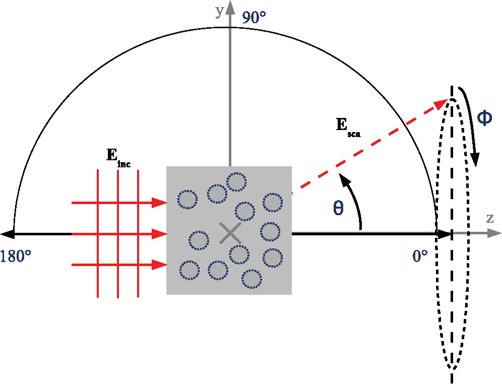 2.1.Monte Carlo ModelA Monte Carlo program for simulation of polarized light propagation in scattering media was developed based on the radiative transfer theory.10,13,15–18,20,21,28 The Monte Carlo method simulates a multitude of random light propagation paths through the medium omitting the wave character of light, nonetheless considering polarization effects. The scatterers were assumed to be randomly distributed within a simulation volume of and to have an angularly-resolved scattering probability (phase function) similar to the phase function of a single sphere. This phase function was calculated using Mie theory (single homogeneous sphere in a homogeneous medium, see Bohren and Huffman32 and Mie33) and used in case of a scattering event. For polarized light, this phase function depends on both the scattering angle as well as on the polarization state of the incident light. The optical properties of polystyrene microspheres (radius ) in water were used as input parameters for the spherical scatterers in the Mie program: the refractive index of the spheres was in an infinite medium of . There was no difference between the refractive index of the medium within the simulation volume and the surrounding medium. The vacuum wavelength of the light was set to . This results in a size parameter . The scattering efficiency of a single sphere resulting from the Mie program can be applied to calculate the scattering coefficient as in Eq. (2) used for the Monte Carlo simulations where the volume of a single sphere , the scattering cross section and the volume fraction (concentration) of spheres in a volume are given. A volume fraction of 5.03 Vol.-% (corresponding to a number of spheres ), 10.05 Vol.-% (), 20.11 Vol.-% () and 40.21 Vol.-% () resulted in a scattering coefficient of , , and , respectively, for the Monte Carlo simulations. The absorption coefficient was set to zero for all concentrations. The number of photons used for the simulations was and , respectively.A commonly used technique to gain the Müller matrix elements of a scatterer system via the Monte Carlo method is the subsequent execution of four simulations applying an incident Stokes vector of , , and which is labeled by H, V, P and R, respectively.6,20 The exit (scattering) angle of each photon which left the simulation volume was registered for each simulation run together with its corresponding Stokes vector. The results are four scattered Stokes vectors : , , and . These four Stokes vectors, resulting from the average of many photon paths, can be used to calculate the Müller matrix of the system: By this method, the angular distribution of each Müller matrix element was obtained. All Müller matrix elements were normalized to the element for each scattering angle and the Müller matrix element was normalized to the element for all angles . The resulting normalized Müller matrix is denoted by in Sec. 3.2.2.Maxwell TheoryA Maxwell solution for the scattering problem is given by the Generalized Multiparticle Mie approach, an extension of Mie theory, which is able to handle multiple spherical scatterers and, as an exact solution, also takes into account dependent scattering effects. A Fortran code is provided by Xu et al.34 and used as a reference Maxwell solver. Therein the scattering of an incident plane wave by a distinct arrangement of spheres is calculated by employing the wave equation as opposed to the statistical Monte Carlo model dealing with photon paths. The total scattered field results from coherent superposition of the scattered field contributions of each sphere : Therein the field scattered by each individual sphere results from an incident field which is composed of the external incident field as well as the scattered fields from all other spheres: The solution of the resulting equation system is described in detail by Xu.30 It yields expansion coefficients for the scattered field containing interaction information of the whole sphere arrangement. This is referred to as dependent scattering. In the far-field, a () complex-valued amplitude scattering matrix can be derived35 for monochromatic incident light which specifies the angular part of the scattered spherical wave’s amplitude distribution. Thus, the scattering problem can be compactly written as32 where the incident plane wave (wavenumber ) propagates along the -axis (see Fig. 1) and the scatterer is located at the origin of the reference frame. For a given scatterer orientation, all elements of this amplitude scattering matrix in Eq. (6) are generally dependent on scattering angle as well as azimuthal angle . In this formulation, the incident and scattered fields consist of parallel and perpendicular components which contain all phase information. Yet, these quantities are sophisticated to interpret in terms of polarized intensities as given in the Stokes vector components. Therefore the elements of the amplitude scattering matrix are converted to particular Müller matrix elements as can be found in Bohren and Huffman:32 Just like the amplitude matrix, all Müller matrix elements in Eq. (7) depend on both scattering angle and azimuthal angle . Thus, to comply with the -dependent Monte Carlo results, each element is azimuthally averaged. In addition, all Müller matrix elements except itself are normalized to to get results within a range of . For ease of comparison, the intensity is normalized to the Monte Carlo solution.Since multiparticle Mie theory requires definitely positioned scatterers of finite extent for solution of the underlying boundary conditions, a collection of spheres is randomly distributed in a given simulation volume in order to achieve defined volume concentrations. To approximate homogeneous turbid media models, several random configurations of finite spheres (realizations) are generated where the results are averaged over these realizations. The spheres are randomly distributed under the restriction that no overlapping is allowed. For generation of these distributions a Metropolis shuffling algorithm36,37 was programmed where each sphere in an initial periodic arrangement (simple cubic lattice) is randomly shuffled many times consi-dering periodic boundary conditions with respect to the cubic volume. This algorithm converges to an equilibrium distribution when performing a high number of displacement steps. In order to improve convergence of the algorithm, the random step size is adjusted dynamically. An initial displacement step size is randomly chosen within a size interval in the order of the sphere radius. After shuffling each sphere for a predefined number of times, an acceptance rate of allowed (non-overlapping) with respect to tried sphere displacements is evaluated. In case the new position would lead to sphere overlap the tried displacement is rejected and the old position is kept.37 A small acceptance rate indicates a poor probability to find allowed positions, then the step size is decreased for the next shuffling pass. On the other hand, a high acceptance rate indicates too small deviation from the initial arrangement, in that case the step size is increased for the next shuffling pass. Generation of sufficiently randomized sphere distributions is achieved if the acceptance rate stays around 50%. For the Maxwell simulations, the same parameters as for the Monte Carlo simulations were used, i.e., the different volume concentrations are modeled by and 96 spheres (), respectively, in a simulation volume of . This volume size allows simulations to be performed in a reasonable amount of time even at higher volume concentrations. Apart from diffraction around forward scattering angles, the characteristics of an infinite scattering medium are reproduced in this subset simulation volume. For the four concentrations 10 distinct random realizations were generated where each sphere is shuffled ca. 10000 times. From these realizations the resulting Müller matrix elements are averaged to reduce interference effects. As above, the incident vacuum wavelength is set to , the relative refractive index to resulting in a size parameter . 2.3.Properties of the Müller MatrixBoth introduced methods are based on scatterers of spherical symmetry. This leads to a reduction in the number of independent Müller matrix elements. Moreover, random orientation of these scatterers has an additional impact on the matrix properties. For example, arbitrarily shaped scatterers of random orientation lead to 10 independent elements. Employing scatterers which have a plane of symmetry further reduces the number of independent elements to 6 (see van de Hulst38). In case of randomly arranged spheres (labeled ), the Müller matrix can be denoted as The off-diagonal elements , , , , , , and vanish. Further, the elements and are symmetric () whereas and are antisymmetric (). All diagonal elements are differing. Note that in case of spheres additional relations38,39 (, ) are only valid if multiple scattering is neglected (single scattering). That means, multiple scattering can be interpreted as violation of spherical symmetry of an equivalent single scatterer.6 These diagonal elements characterize the coupling of equal Stokes components by the scattering system. The element shows the degree of parallel linear polarization with respect to unpolarized incident light whereas shows the transformation of oblique linear to circular polarization. From the Müller matrix elements information on the conservation of interference effects40 and polarization states41 can be derived. For spheres with high relative refractive index it is known that depending on the scatterers’ size parameter residing in Rayleigh or Mie regime, linear or circular polarization states are better maintained, respectively.5,423.Results and DiscussionThe resulting 16 angularly resolved Müller matrix elements were compared between the Monte Carlo method and the Maxwell method. Figure 2 shows all angularly resolved Müller matrix elements in case of 24 randomly distributed spheres corresponding to a volume concentration .-%. It is obvious that both submatrices on the secondary diagonal [see Eq. (8), namely the , , , , , , and elements] show noisy results around zero for all angles. This behavior was expected for single as well as for multiple scattering by randomly distributed spheres.38 Further, the well-known symmetry between the and elements as well as antisymmetry between the and elements was reproduced by both methods. The remaining concentrations of 12 (.-%), 48 (.-%) and 96 spheres (.-%) dispersed in the medium showed the same expected behavior as above. Because of that, only the relevant Müller matrix elements , , , and , are shown in Fig. 3 (12 spheres), Fig. 4 (48 spheres) and Fig. 5 (96 spheres). Fig. 2Angularly resolved Müller matrix: Monte Carlo results (red) and Maxwell results (black) compared to each other. Parameters used: nonabsorbing spheres (radius , relative refractive index ), size of cubic scattering volume (volume concentration .-%), wavelength of incident light in vacuo. All elements are normalized to , the element is normalized to forward direction. Every element is depicted versus the scattering angle in the range from 0 to 180 deg.  Fig. 3Relevant Müller matrix elements for nonabsorbing spheres (.-%). All elements are normalized to , the element is normalized to forward direction. Every element is depicted versus the scattering angle in the range from 0 to 180 deg.  Fig. 4Relevant Müller matrix elements for nonabsorbing spheres (.-%). All elements are normalized to , the element is normalized to forward direction. Every element is depicted versus the scattering angle in the range from 0 to 180 deg. Increasing deviations due to dependent scattering can be observed. 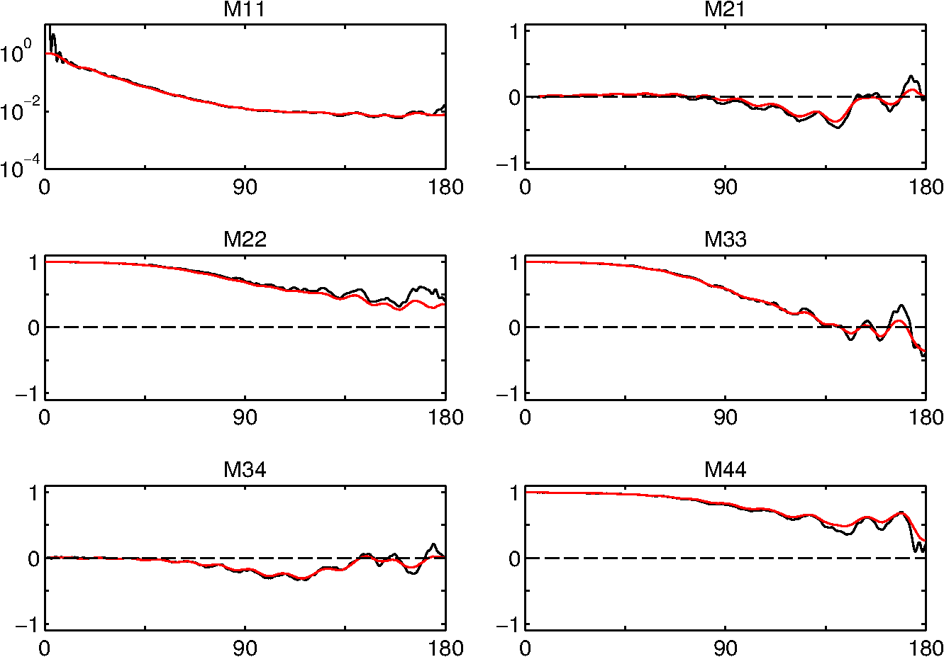 Fig. 5Relevant Müller matrix elements for nonabsorbing spheres (.-%). All elements are normalized to , the element is normalized to forward direction. Every element is depicted versus the scattering angle in the range from 0 to 180 deg. Deviations due to dependent scattering are obvious. 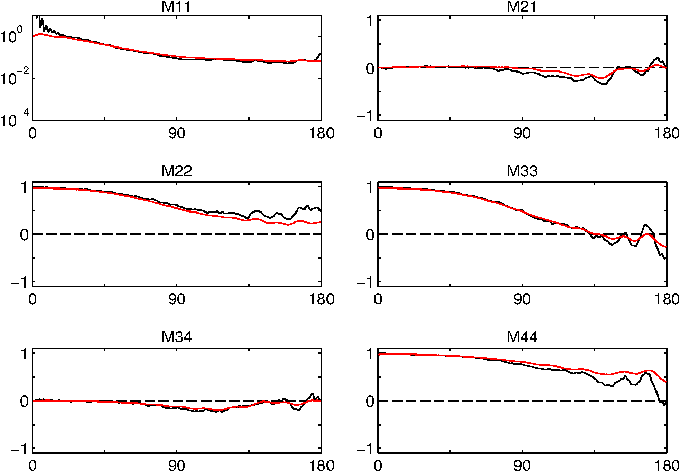 3.1.Effects on Multiple and Dependent ScatteringThis study was aimed at pointing out agreements and differences between the two light scattering simulation approaches for polarized light. It can be observed that especially for small concentrations the two methods are in good agreement for all Müller matrix elements. This was already described for unpolarized light27 and was now observed for polarized light within this study.28 With increasing scatterer concentrations slightly increasing differences can be observed for all Müller matrix elements, mainly for higher scattering angles. These differences are attributed to dependent scattering effects since multiple scattering is considered by both solution methods. In Fig. 6 the angular errors are depicted for the same Müller matrix elements as above and three different volume concentrations. For the relative error and for all normalized elements the difference between the both methods is shown. Only for large investigated volume concentrations above 20 Vol.-% dependent scattering effects become predominant, especially in the backscattering hemisphere. It is not possible to reproduce dependent scattering by standard solutions of the radiative transfer theory due to near field interactions. This has to be kept in mind whenever results of Monte Carlo simulations of polarized light propagation are regarded. Fig. 6Concentration dependent deviations between Maxwell and Monte Carlo results for all relevant Müller matrix elements. In case of the relative error is calculated, otherwise the difference between normalized elements. For volume concentrations of .-% (red), .-% (blue) and .-% (black) the resulting deviations are depicted versus the scattering angle in the range from 0 to 180 deg. Apart from forward- and backscattering peaks () deviations do not exceed 30%. 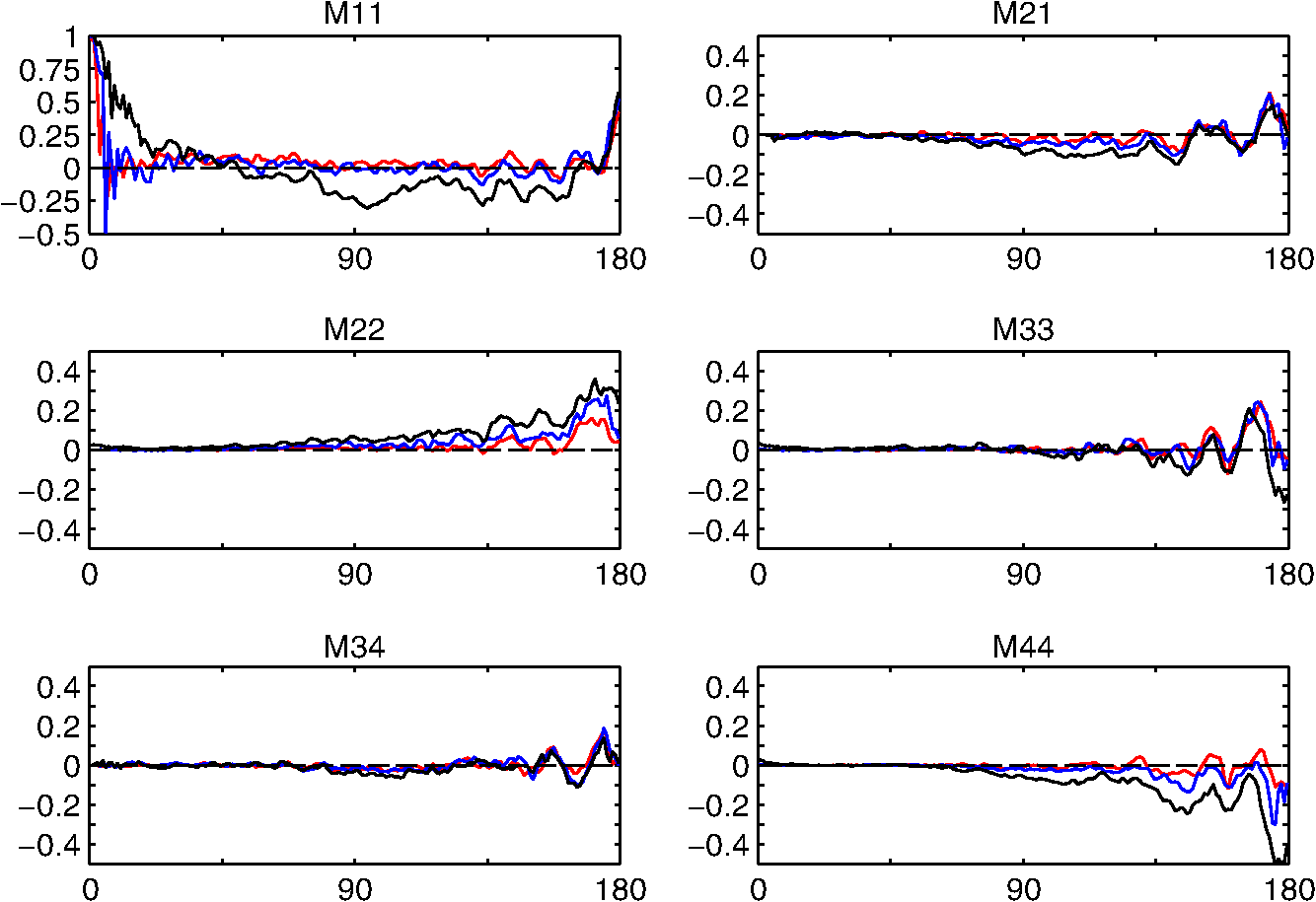 All Müller matrix elements show oscillations in the whole angular range, especially for small concentrations, while the oscillations are decreasing with increasing scatterer concentrations. These oscillations for small concentrations result from the solution of scattering by a single sphere (Mie scattering). With increasing concentrations, multiple scattering becomes predominant which leads to a reduction of the oscillation amplitudes. 3.2.Results for the Unpolarized IntensityThe element is a normalized measure for the scattered intensity for unpolarized light. The differences in the element between the two methods for small angles () are due to forward interferences resulting from the limited simulation volume (Maxwell theory).27 The angular width of these forward interferences would become infinitesimally small if a laterally infinite instead of a finite cubic simulation volume would be regarded. Another effect is the coherent backscattering peak43 at which can be reproduced by Maxwell theory in contrast to the radiative transfer theory. It can be observed for all concentrations and for scattering angles near and becomes more pronounced for high scatterer concentrations. Forward interferences and coherent backscattering cannot be reproduced by the Monte Carlo method as the radiative transfer theory neglects the wave character of light. Beside that, it can be observed that the angular distribution of the element flattens for higher sphere numbers, i.e., the scattered intensity becomes more isotropic with increasing concentrations. This effect appears for both methods. Further, a flattening of the oscillations attributed to the single Mie scattering function is found for higher concentrations, also for the other Müller matrix elements. Increasing concentrations lead to irregular deviations of the element between both methods being most apparent for the highest concentration (96 spheres). The Monte Carlo solution stays rather smooth while the exact Maxwell results show more oscillations, even if no speckles are considered. 3.3.Polarization Specific Müller Matrix ElementsThe absolute value of all normalized Müller matrix elements (except ) generally decreases for higher angles as the concentration increases. This effect, investigated with Monte Carlo simulations, was attributed to multiple scattering by Tuchin et al.6 The Maxwell solutions presented here show a similar behavior even if increasing deviations to the Monte Carlo solutions for higher concentrations are taken into account. The decrease of these Müller matrix elements indicates the depolarizing character of multiple scattering. It is important to mention that the described decrease is mostly present, though for some angles there are also exceptions of this behavior. For angles near forward direction, the , and elements take values near 1, while the off-diagonal elements take values near 0 for all concentrations. This means that the polarization properties are better maintained in the forward direction. For both simulation methods this effect is dominant for small concentrations. The element contains information about the circular polarization. It also decreases when scatterer concentrations increase for forward scattering angles , but the decrease is smaller than for the and Müller matrix elements. For higher scattering angles, no general decrease with higher concentrations of the element can be observed from the Monte Carlo simulations. It could be confirmed that this effect can mainly be attributed to multiple scattering as was assumed by Maksimova et al.,18 who considered constant scatterer concentrations (size parameters in the Mie regime), but increasing scattering volumes. This may indicate that circular polarization is better maintained than linear polarization for multiple scattering. However, for very high scatterer concentrations as is the case for 96 spheres dispersed in the medium it can be observed (see Fig. 5) that the element calculated by Maxwell theory is below the element calculated by the Monte Carlo method while the element shows an opposite behavior. This shows that the better maintenance of circular polarization for high scatterer concentrations is not as manifest as could be expected only due to multiple scattering. In this case dependent scattering leads to a further reduction of the element. It has to be mentioned that these results hold for the parameters used in this study with scatterers in the Mie regime and a relatively high refractive index mismatch between scatterer and surrounding medium. For scattering media in the Rayleigh regime or in the Mie regime in case of scatterers with low relative refractive index it is possible that linear polarization is better maintained than circular polarization.5 4.ConclusionsIn summary it could be shown that it is possible to reproduce the exact Maxwell solutions for low to moderate volume concentrations in good approximation when using a polarization sensitive Monte Carlo code based on radiative transfer theory. This holds for all Müller matrix elements, especially for scattering angles . For high volume concentrations of the scatterers (.-% in this study), dependent scattering effects are no longer negligible, so in case of highly concentrated scatterers the results of the Monte Carlo method must be taken with care, especially for high scattering angles. The direct comparison method between solutions of the radiative transfer theory and Maxwell theory for the whole Müller matrix is useful for testing polarization dependent Monte Carlo programs for arbitrary optical properties of the scatterers and the surrounding medium. This could lead to more realistic simulation models of biological tissue. An extended investigation for complex models including polydisperse and absorbing scatterers, as is the case for biological media, is expected to disclose more polarization features. AcknowledgmentsWe acknowledge support of the Deutsche Forschungsgemeinschaft (DFG grant KI 538/14-1). ReferencesH. Dinget al.,
“Angle-resolved Mueller matrix study of light scattering by B-cells at three wavelengths of 442, 633, and 850 nm,”
J. Biomed. Opt., 12
(03), 034032
(2007). http://dx.doi.org/10.1117/1.2749730 JBOPFO 1083-3668 Google Scholar
Y. Liuet al.,
“Optical markers in duodenal mucosa predict the presence of pancreatic cancer,”
Clin. Cancer Res., 13
(15), 4392
–4399
(2007). http://dx.doi.org/10.1158/1078-0432.CCR-06-1648 1078-0432 Google Scholar
J. C. Ramella-RomanA. NayakS. A. Prahl,
“Spectroscopic sensitive polarimeter for biomedical applications,”
J. Biomed. Opt., 16
(04), 047001
(2011). http://dx.doi.org/10.1117/1.3561907 JBOPFO 1083-3668 Google Scholar
B. V. Bronket al.,
“Measuring diameters of rod-shaped bacteria in vivo with polarized light scattering,”
Biophys. J., 69
(3), 1170
–1177
(1995). http://dx.doi.org/10.1016/S0006-3495(95)79991-X BIOJAU 0006-3495 Google Scholar
N. GhoshI. Vitkin,
“Tissue polarimetry: concepts, challenges, applications, and outlook,”
J. Biomed. Opt., 16
(11), 110801
(2011). http://dx.doi.org/10.1117/1.3652896 JBOPFO 1083-3668 Google Scholar
V. TuchinL. WangD. Zimnyakov, Optical Polarization in Biomedical Applications, 1 Springer, Berlin
(2006). Google Scholar
C. ChuS. Churchill,
“Multiple scattering by randomly distributed obstacles—methods of solution,”
IEEE Trans. Antenn. Propag., 4
(2), 142
–148
(1956). http://dx.doi.org/10.1109/TAP.1956.1144373 IETPAK 0018-926X Google Scholar
B. WilsonG. Adam,
“A Monte Carlo model for the absorption and flux distributions of light in tissue,”
Med. Phys., 10
(6), 824
–830
(1983). http://dx.doi.org/10.1118/1.595361 MPHYA6 0094-2405 Google Scholar
M. Antonelliet al.,
“Mueller matrix imaging of human colon tissue for cancer diagnostics: how Monte Carlo modeling can help in the interpretation of experimental data,”
Opt. Express, 18
(10), 10200
–10208
(2010). http://dx.doi.org/10.1364/OE.18.010200 OPEXFF 1094-4087 Google Scholar
S. BartelA. Hielscher,
“Monte Carlo simulations of the diffuse backscattering Mueller matrix for highly scattering media,”
Appl. Opt., 39
(10), 1580
–1588
(2000). http://dx.doi.org/10.1364/AO.39.001580 APOPAI 0003-6935 Google Scholar
B. CameronY. LiA. Nezhuvingal,
“Determination of optical scattering properties in turbid media using Mueller matrix imaging,”
J. Biomed. Opt., 11
(05), 054031
(2006). http://dx.doi.org/10.1117/1.2363347 JBOPFO 1083-3668 Google Scholar
A. Hielscheret al.,
“Diffuse backscattering Mueller matrices of highly scattering media,”
Opt. Express, 1
(13), 441
–453
(1997). http://dx.doi.org/10.1364/OE.1.000441 OPEXFF 1094-4087 Google Scholar
M. J. Rakovićet al.,
“Light backscattering polarization patterns from turbid media: theory and experiment,”
Appl. Opt., 38
(15), 3399
–3408
(1999). http://dx.doi.org/10.1364/AO.38.003399 APOPAI 0003-6935 Google Scholar
H. AkarçayJ. Ricka,
“Simulating light propagation: towards realistic tissue models,”
Proc. SPIE, 8088
(1), 80880K
(2011). http://dx.doi.org/10.1117/12.889135 PSISDG 0277-786X Google Scholar
D. CôtéI. Vitkin,
“Robust concentration determination of optically active molecules in turbid media with validated three-dimensional polarization sensitive Monte Carlo calculations,”
Opt. Express, 13
(1), 148
–163
(2005). http://dx.doi.org/10.1364/OPEX.13.000148 OPEXFF 1094-4087 Google Scholar
X. GuoM. WoodA. Vitkin,
“A Monte Carlo study of penetration depth and sampling volume of polarized light in turbid media,”
Opt. Commun., 281
(3), 380
–387
(2008). http://dx.doi.org/10.1016/j.optcom.2007.09.043 OPCOB8 0030-4018 Google Scholar
G. KattawarC. Adams,
“Stokes vector calculations of the submarine light field in an atmosphere-ocean with scattering according to a Rayleigh phase matrix: effect of interface refractive index on radiance and polarization,”
Limnol. Oceanogr., 34
(8), 1453
–1472
(1989). http://dx.doi.org/10.4319/lo.1989.34.8.1453 LIOCAH 0024-3590 Google Scholar
I. L. MaksimovaS. RomanovV. Izotova,
“The effect of multiple scattering in disperse media on polarization characteristics of scattered light,”
Opt. Spectrosc. (USSR), 92
(6), 915
–923
(2002). http://dx.doi.org/10.1134/1.1490031 OPSUA3 0030-400X Google Scholar
M. Xu,
“Electric field Monte Carlo simulation of polarized light propagation in turbid media,”
Opt. Express, 12
(26), 6530
–6539
(2004). http://dx.doi.org/10.1364/OPEX.12.006530 OPEXFF 1094-4087 Google Scholar
J. Ramella-RomanS. PrahlS. Jacques,
“Three Monte Carlo programs of polarized light transport into scattering media: part I,”
Opt. Express, 13
(12), 4420
–4438
(2005). http://dx.doi.org/10.1364/OPEX.13.004420 OPEXFF 1094-4087 Google Scholar
X. WangL. Wang,
“Propagation of polarized light in birefringent turbid media: a Monte Carlo study,”
J. Biomed. Opt., 7
(3), 279
–290
(2002). http://dx.doi.org/10.1117/1.1483315 JBOPFO 1083-3668 Google Scholar
A. TafloveS. Hagness,
“Computational electrodynamics: the finite-difference time-domain method,”
Artech House Antennas and Propagation Library, Artech House, Boston
(2005). Google Scholar
B. DraineP. Flatau,
“Discrete-dipole approximation for scattering calculations,”
JOSA A, 11
(4), 1491
–1499
(1994). http://dx.doi.org/10.1364/JOSAA.11.001491 JOAOD6 1084-7529 Google Scholar
S. H. TsengB. Huang,
“Comparing Monte Carlo simulation and pseudospectral time-domain numerical solutions of Maxwell’s equations of light scattering by a macroscopic random medium,”
Appl. Phys. Lett., 91
(5), 051114
(2007). http://dx.doi.org/10.1063/1.2767777 APPLAB 0003-6951 Google Scholar
J. SchäferA. Kienle,
“Scattering of light by multiple dielectric cylinders: comparison of radiative transfer and Maxwell theory,”
Opt. Lett., 33
(20), 2413
–2415
(2008). http://dx.doi.org/10.1364/OL.33.002413 OPLEDP 0146-9592 Google Scholar
L. Rouxet al.,
“Scattering by a slab containing randomly located cylinders: comparison between radiative transfer and electromagnetic simulation,”
JOSA A, 18
(2), 374
–384
(2001). http://dx.doi.org/10.1364/JOSAA.18.000374 JOAOD6 1084-7529 Google Scholar
F. VoitJ. SchäferA. Kienle,
“Light scattering by multiple spheres: comparison between Maxwell theory and radiative-transfer-theory calculations,”
Opt. Lett., 34
(17), 2593
–2595
(2009). http://dx.doi.org/10.1364/OL.34.002593 OPLEDP 0146-9592 Google Scholar
A. Hohmannet al.,
“Comparison of Monte Carlo simulations of polarized light propagation in turbid media with exact Maxwell solutions,”
Proc. SPIE, 8090
(1), 80900H
(2011). http://dx.doi.org/10.1117/12.889349 PSISDG 0277-786X Google Scholar
A. Kienleet al.,
“Light propagation in dentin: influence of microstructure on anisotropy,”
Phys. Med. Biol., 48
(2), N7
–N14
(2003). http://dx.doi.org/10.1088/0031-9155/48/2/401 PHMBA7 0031-9155 Google Scholar
Y. Xu,
“Electromagnetic scattering by an aggregate of spheres,”
Appl. Opt., 34
(21), 4573
–4588
(1995). http://dx.doi.org/10.1364/AO.34.004573 APOPAI 0003-6935 Google Scholar
J. Hovenier,
“Structure of a general pure Mueller matrix,”
Appl. Opt., 33
(36), 8318
–8324
(1994). http://dx.doi.org/10.1364/AO.33.008318 APOPAI 0003-6935 Google Scholar
C. BohrenD. Huffman, Absorption and Scattering of Light by Small Particles, Wiley-Interscience, New York
(1998). Google Scholar
G. Mie,
“Beiträge zur Optik trüber Medien, speziell kolloidaler Metallösungen,”
Ann. Phys., 330
(3), 377
–445
(1908). http://dx.doi.org/10.1002/(ISSN)1521-3889 ANPYA2 0003-3804 Google Scholar
Y. XuB. Gustafson,
“An analytical solution to electromagnetic multisphere-scattering,”
(2003) http://www.scattport.org/files/xu/codes.htm Google Scholar
Y. Xu,
“Scattering Mueller matrix of an ensemble of variously shaped small particles,”
JOSA A, 20
(11), 2093
–2105
(2003). http://dx.doi.org/10.1364/JOSAA.20.002093 JOAOD6 1084-7529 Google Scholar
N. Metropoliset al.,
“Equation of state calculations by fast computing machines,”
J. Chem. Phys., 21
(6), 1087
–1092
(1953). http://dx.doi.org/10.1063/1.1699114 JCPSA6 0021-9606 Google Scholar
L. Tsanget al., Scattering of Electromagnetic Waves: Numerical Simulations, 2 Wiley-Interscience, New York
(2001). Google Scholar
H. Van de Hulst, Light scattering by Small Particles, 1 Dover Publications, New York
(1981). Google Scholar
M. HoferO. Glatter,
“Mueller matrix calculations for randomly oriented rotationally symmetric objects with low contrast,”
Appl. Opt., 28
(12), 2389
–2400
(1989). http://dx.doi.org/10.1364/AO.28.002389 APOPAI 0003-6935 Google Scholar
M. MishchenkoD. Mackowski,
“Coherent backscattering in the cross-polarized channel,”
Phys. Rev. A, 83
(1), 013829
(2011). http://dx.doi.org/10.1103/PhysRevA.83.013829 PLRAAN 1050-2947 Google Scholar
S. Savenkov,
“Mueller-matrix characterization of biological tissues,”
Polarimetric Detection, Characterization and Remote Sensing, 437
–472 Springer, Dordrecht
(2011). Google Scholar
D. Bicoutet al.,
“Depolarization of multiply scattered waves by spherical diffusers: influence of the size parameter,”
Phys. Rev. E, 49
(2), 1767
–1770
(1994). http://dx.doi.org/10.1103/PhysRevE.49.1767 PLEEE8 1539-3755 Google Scholar
M. MishchenkoL. TravisA. Lacis, Multiple Scattering of Light by Particles: Radiative Transfer and Coherent Backscattering, Cambridge Univ. Press, New York
(2006). Google Scholar
|


