|
|
1.IntroductionThe genetic regulation mechanisms of cells are composed of many interacting complex, dynamical networks. The networks that control cell growth, differentiation, maintenance, repair, and many other functions of an adult organism, are essentially nonlinear types of process control. The structure of these networks contains parallel, or intertwining, pathways that have various inputs, outputs, loops, and cross-talks with each other. These levels of nonlinearity of the network guarantee that there are highly consequential, intermittently functioning operations that are only observable while the system experiences a shift in the operating regulatory dynamics in response to particular influences. The traditional reductionist approach that only focuses on a specific regulatory unit fails to capture the full dynamics of the system. Some high-throughput techniques like RNA expression profiling with microarrays can provide a snapshot of an aspect of the system at one time point, but to follow cell responses for an extended period by microarrays, one needs to carefully prepare multiple cell populations under identical conditions and produce the assays at different time points by harvesting cells and extracting analyte from a different cell population at each time point. The whole procedure is technically cumbersome and error-prone, and the cost can be prohibitive if dense temporal sampling is carried out. Fluorescent reporters have long been used in molecular technology to study cells transcriptional activities, the cellular localization of components, or re-distribution of target proteins, either in a population of cells or a single cell.1–3 There are two basic types of fluorescent reporters based on the molecular structure: (1) Promoter-reporters that indicate the activity of the promoter for a particular gene. To serve this purpose, a fluorescent reporter can be constructed by fusing the promoter region of a gene of interest with the coding sequence of a fluorescent protein, most commonly a green fluorescent protein (GFP). Then the abundance of the reporter can be used as an indicator of the activity of the promoter. (2) Fusion-reporters that indicate the cellular location of a protein, the stability of a protein, the status of large architectural elements in the cell, or the positioning of small molecules in a cell. This type of fluorescent reporter is made by an in-frame fusion of the coding sequence of either a whole protein or a protein domain to the coding sequence of a fluorescent protein, and then placing that coding sequence under the control of a promoter that will drive the production of that protein at a rate sufficient to produce constant detectable levels of the fusion protein. The presence of fluorescent molecules can be detected by imaging with an epifluorescent microscope. Because this procedure is non-invasive to the cell, it allows tracking of the same cell population for an extended period of time by imaging the same site repeatedly. The recent introduction of automated digital microscopes allows researchers to use multi-well microtiter plates and sequentially capture the reporter activities in all wells in a high-content fashion.4–6 To the present day, the majority of approaches that take advantage of such large-scale fluorescent imaging assays limit themselves to the fusion reporters, where the dynamic spatial distributions of such fusion-proteins serve as the indicators of phenotypes of interest. These fusion-reporters can be used in large scale RNAi or small molecules screening, in time-lapse study and/or case-control study.7–11 However, to serve as phenotype indicators, only a few key reporters are needed, often less than three. Hence such approaches provide little insights on the mechanism of the cellular regulation network in response to external perturbations. In this study, we used a batch of promoter reporters to track the transcriptional activities of particular genes. To serve this purpose, we built a library of promoter reporters and designed an experimental protocol. In our experimental protocol, a single assay is carried out by epifluorescent imaging of a site at the bottom of each well in a 384-well plate, producing an image of the cells in that region (∼200 to 300 cells) bearing fluorescent reporters. The imaging speed of automated systems easily accommodates sampling an entire 384-well plate at hourly intervals. If needed, the experiment can be extended to multiple sites/plates to cover more cells with a wider range of cell types and reporters. Using different wells to test different combinations of cell type, GFP reporter and experimental conditions allows this innovative approach to provide a truly multi-dimensional examination of the cell’s responses to a variety of stimuli. Not only can it follow multiple genes simultaneously, but it can also compare cellular activities under various conditions. Furthermore, it captures the dynamics of transcriptional regulation. The capability to observe a cohort of cell-response behaviors facilitates new possibilities in biological research, e.g., detection of sub-populations with different susceptibilities to the external stimuli, determination of whether the response is continuous or graded, ordering of critical events, and relating different response patterns. To fully realize these possibilities and explore the potential of this method in biological and pharmaceutical applications, we have designed a customized data processing procedure for this experimental protocol. The procedure contains two parts: (1) image processing and transcription quantification, where the fluorescent images are segmented to identify individual nuclei and cells, and the amount of fluorescence each cell is producing is quantified, and (2) data representation, where the extracted time course data are summarized and represented in a way that can facilitate efficient evaluation. 2.MethodsSince the proposed data processing procedure is designed for a high-content fluorescent protein reporter-based experimental protocol, it is necessary to provide some basic information on how the experiment is carried out and the unique challenges associated with the protocol. 2.1.Experimental ProtocolThe objective of the experimental protocol is to efficiently capture cell process dynamics in response to certain stimuli in order to obtain a deeper understanding of the genetic regulatory mechanisms and constrain the number of possible mechanisms requiring further research. For example, the stimuli applied could be chemicals, biological molecules or environmental alterations. The design and execution of experiments are aimed at understanding the mechanisms invoked in response to a stimulus, and is generally carried out in the three stages: (1) formulate a model of pathways on the processes potentially affected by the stimulus, pick the desired process reporters and cell lines based on the model, and prepare and plate sets of cell line/reporter pairs; (2) perturb the pathways with the stimulus of interest and other stimuli with known effects on components of the pathways of interest, and also include an un-stimulated control; and (3) take fluorescent images periodically for a consecutive time period for all cell populations in the plate. The fluorescent images are taken as two-color image pairs with a blue channel image for the nuclei and a green channel image for the GFP reporters. The imaging rate should be frequent enough to capture any change in the transcription activity, yet not too frequent to induce photobleaching and/or phototoxicity. The transcription itself is a slow, yet dynamic process. It can take 4 to 6 h or more from the time transcription rates change to the time when the new steady-state level of protein product is achieved. Moreover, the protein product is in continuous turnover through translation and proteolysis. The microscope has been fitted with several filters in case that the target cell line is sensitive to light at certain frequency. One can switch to other color channels by using filters in combination with other fluorescent reporters or stains, and avoid or alleviate potential toxic effects. Finally, the computer-controlled shutters used by the automatic imager greatly limit the exposure time of live cells, which further prevents phototoxicity. Thus, we found an hourly sampling rate is sufficient for successful transition tracking, yet low enough not to induce any observable photobleaching and phototoxicity. In a properly designed plate, each condition will be tested in multiple wells to ensure both adequate coverage and replicates to assess technical variation. In our experiments, every condition is duplicated in three or more wells. There will also be media-only, unperturbed cell population to serve as negative controls and cell-lines with a highly expressed reporter to serve as positive controls. These control wells can serve as a final safeguard to detect any unexpected effects. In the beginning of the experiment, the plate will be imaged for several hours without any stimulants being added. The images taken during this period will provide an estimate on the baseline level of transcriptional activity. Once the stimulants are added, the images will be taken hourly for considerable time, usually over 40 h, to capture any induced response by the chosen reporters. The technical details on how the biological samples were prepared and how the images were taken are available in the Appendix. Figure 1 shows two typical fluorescent images sampled for the same site in a 48-h drug treatment study. The original images are 16-bit images and are normalized to 8-bit for proper viewing. The full sequence of images is stacked into a video file. The colon cancer cell-line HCT116 is under observation here and the reporter is driven by a 1 kb promoter fragment from MKI67, a nuclear protein whose abundance is tightly correlated with proliferation.12 No drug was added for the first 5 h, then lapatinib, a drug used to treat breast cancer, was added and imaged for 43 h. In Fig. 1, the left image was taken at the beginning of the experiment when no drug has been added, while the right image was taken 43 h after the drug lapatinib was added. There are about 300 cells in the image. The nuclear channel (blue) images the live cell DNA fluorophore, Vybrant Violet, and the promoter reporter activity channel (green) images the GFP reporter protein. For the case shown here, the change in transcriptional activity is significant. In the beginning, gene MKI67 is highly transcribed, indicating strong proliferation activity. At the end of the experiment, most of the GFP fluorescence was reduced to almost unobservable, a likely indicator of reduced transcription followed by apoptotic proteolysis. Fig. 1Two fluorescent images of the same imaging site for cell-line HCT116 with a promoter reporter for the gene MKI67 taken in the time course of one experiment: (a) before any drug is applied (beginning of Video 1); (b) 43 h after a drug lapatinib was added (end of Video 1). (Video 1, QuickTime, MOV, 2.6 MB). [URL: http://dx.doi.org/10.1117/1.JBO.17.4.046008.1].  Figure 1 shows that fluorescent reporters can help researchers track the cellular activity of the same cohort of cells, in this case, by direct visual evaluation; however, the volume of data that can be handled by visual inspection in a timely manner is very limited, while the volume of data generated by the current approach is always huge. With a 384-well plate there will be 384 videos for evaluation and the number can be much higher if the experiment requires multiple sites being chosen in each well or multiple plates to cover all experimental conditions. Furthermore, visual evaluation is unreliable when one needs to aggregate the results from duplicated wells or when one needs to quantitatively compare different conditions. Hence the high-content nature of the GFP reporter approach calls for a more automatic and quantitative solution to efficiently extract and summarize the captured transcriptional activity. 2.2.Image Processing2.2.1.Objectives of image processingTo facilitate automatic processing of the experiment results, the first step is image processing, where the transcriptional levels of the fluorescent images will be properly extracted, quantified, and saved. When designing the image processing method, several characteristics of cell imaging specific to the experimental protocol must be considered.
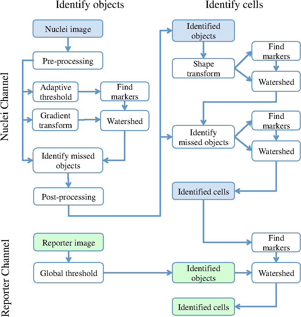
2.2.2.Image processing procedureAchieving all of these objectives requires a fast image processing algorithm with good balance between speed and the ability to pick up almost all objects. The most common segmentation methods involve an adaptive-threshold-based approach like the one based on the top-hat transform.15 We have found this approach, with a properly chosen threshold, to be fast and able to identify the foreground objects in general for almost all cases. However, it is difficult to find the optimal threshold for such an approach, which makes it hard to further identify individual nuclei. Level-set-based methods are another popular approach that has been reported to achieve impressive performances, but can be quite complicated and time-consuming.16–18 For our experiments, we found that the potential performance gain through this approach does not compensate for the extra computation time and complexity. We decided to build our method using morphological image processing,15 in particular, the watershed transformation,19 another popular and proven approach in cellular image processing. The time-course images are processed independently to maintain process speed and minimize the consequence of unexpected outliers: only one pair of images will be loaded and processed each time, and the results of outlier images can later be discarded without affecting other results. Figure 2 provides the general flowchart on how a fluorescent image pair is processed: the nuclear channel is first processed to identify all nuclei (top part of Fig. 2) and the reporter channel is then analyzed to extract an individual cell’s expression activity (bottom part of Fig. 2). As a practical example, the critical steps in processing the image in Fig. 1(a) are shown in Fig. 3. In order to show the segmentation details, only a portion of the full image is shown here. Fig. 3The segmentation of Fig. 1(a): (a) raw image of nuclear channel; (b) markers for gradient-image-based watershed segmentation, where the white dots are the foreground markers, while the white lines are the boundary of background markers; (c) identified foreground region; (d) markers for nuclei de-clumping, the white dots are found by shape information, while the relatively large grey objects are markers found by intensity; the de-clumping is limited to the foreground region defined by the white boundary lines; (e) final segmentation of the nuclei channel; (f) reporter channel, where the white lines are the identified cell boundaries while the grey lines identify the nuclei used as markers.  Nuclear channel processing contains two major steps. First, the foreground objects are identified, where an object is either an isolated nucleus or a cluster of nuclei (top left part of Fig. 2). Before segmentation, the nuclear channel image is first pre-processed to remove tiny additive and subtractive noise via a single-stage open-close alternating sequential filter. We apply watershed-based segmentation on the gradient image. It is known that the accuracy of flood holes is critical to the success of the watershed procedure. As is commonly done, we depend on the top-hat transform for marker selection. The local maxima inside the top-hat-identified foreground are filtered by the area open operation20 to form the foreground markers of size no smaller than a designated value based on common nuclei sizes. Similarly, the background markers are found by morphologically thinning the top-hat identified background. Thinning, rather than erosion, is chosen to avoid small and/or narrow passage regions between nuclei being lost. An example of the watershed markers can be viewed in Fig. 3(b). Overall, the watershed on a gradient image gives a tight boundary on most nuclei; however, if a dim nucleus is attached to a bright nucleus or part of a nucleus is much brighter than other parts, the high gradient of the bright one might overshadow the dim one and the watershed segmentation could miss the dim region. To address this problem, the difference between top-hat transform and watershed results is used to identify and recover large missing objects. To obtain the final identified foreground objects, the segmentation results are sent for post-processing to remove tiny objects that can be artifacts or nuclear debris. An example of the final foreground can be found in Fig. 3(c). The next step is to identify individual nuclei by de-clumping the clustered nuclei (top right part of Fig. 2). In most cases, nuclei have circular or near-circular shapes, and the tight segmentation boundaries secured by the previous step make it a natural choice to use a shape-based de-clumping method, where we apply watershed segmentation on distance transformed foreground images. The local maxima found through morphological opening are set as markers for flooding holes. For the highly clustered regions, where the boundary shape is not informative enough, shape-based de-clumping might fail to separate some or all of the nuclei. These missed objects usually have a much larger area size and irregular shape than can be detected by the circularity shape factor. Intensity-based watershed segmentation is applied to further de-clump these missed objects, where the markers are found through the area open operator. An example of the watershed markers can be found in Fig. 3(d). To save space, we put both shape-based and intensity-based de-clumping markers in one image. Before passing the identified nuclei to the GFP channel processor, a final post-processing is done by removing the tiny objects generated by the de-clumping procedure. An example of the final segmentation results can be found in Fig. 3(e). The parameters associated with image processing must be adjusted for each cell-line and experiment because critical factors associated with segmentation, like nuclei size, shape, and intensity range, can vary significantly due to experiment design, biological diversity, or imaging setting. In some extreme cases, the whole de-clumping part might be omitted if the nuclei do not have a round shape. Indeed, for certain cancer cell-lines, it is common to see large cells with large and/or irregularly shaped nuclei. For example, the breakage-fusion-bridge cycles can create very large nuclei or connected nuclei linked through anaphase or chromatin bridges.21 These irregular nuclei cannot be separated by standard criteria like shape or intensity, and can be ambiguous to determine even by experienced biologists. Hence, for such cases, to avoid further complication, it is better to skip the de-clumping step and treat the identified objects as nuclei. As with the nuclear channel, the processing of the GFP reporter channel can be viewed as a two-step procedure: first, identify the objects; second, identify the cells. Here, both steps are much simpler than their counterparts in nuclear channel. Since the reporters are not bound to any other molecule, one would expect that the fluorescent reporter protein, once produced, should be all over the cytoplasm and quite evenly distributed. Thus, a global threshold can be used to find the objects that have fluorescent intensity over a designated value. The threshold is a fixed value offset by the background intensity, which is largely additive noise that should not be measured as part of the transcriptional activity. The background intensity can be retrieved by finding the mode in the lower part of the intensity histogram. If the cells are at a density where they essentially cover the entire bottom surface of the well, then the mode estimate of the background intensity could be false. In such a case, the imaging site will either be discarded during the quality check or an alternative approach will be used. The reference sites, which have the same media but no cells and are in the same plate, can be used to find the background intensity.* To de-clump the objects into cells, intensity-based watershed segmentation was used. Since the nuclei must be contained in the cells, it is natural to use the identified nuclei as the markers of the presence of a cell for the watershed segmentation. An example of the final GFP reporter channel segmentation results can be found in Fig. 3(f). It should be noted that although we treat the background noise as additive, there exist some multiplicative noise types. Such noise is only prominent when the overall intensity distribution range changes significantly, which can be detected when one observes a large background intensity change. In such cases, rather than trying to normalize such a variance, we discard the site and omit it in the following analysis. Once the individual cells are identified, the transcriptional activity represented by the reporter is extracted for every cell by summing up the background subtracted pixel intensity of the whole cell area and taking a transform before being exported. The transform is taken because the changes of the chemical reactions prevalent in the cells are multiplicative rather than additive and the -transformed intensity can therefore better represent the dynamics of reporter abundance changes in the cell. The results are exported as a tabular data file for further processing. It should be noted that in our study, the transcription activity is collected from the reporter channel, while the nuclei channel only serves an auxiliary role for better segmentation. However, since the morphological changes of the nuclei can also reveal important information on cellular response, we are working on incorporating such information into our protocol. The whole image processing procedure is done with MATLAB, with most morphological operators done by the SDC Morphology Toolbox for MATLAB.15 For a standard image pair of size , with about 300 cells, it takes about five minutes to process a 48-time-point series, which is about 6 s per image pair for a standard Windows-based desktop computer (3.3 GHz processor, 4 GB RAM). By splitting the plate into several blocks and running the program in parallel, a single plate can be processed overnight by a multi-core desktop computer.† 2.3.Data RepresentationOnce the images are processed, transcriptional activity extracted, and the results exported, organized data representation is required to help researchers evaluate the quality of the experiment, investigate the outcome, and identify the biologically meaningful relationships. 2.3.1.Quality controlBefore any further processing of the results, their qualities must be thoroughly examined. The experiments require a great deal of handling, dilutions and delivery of cultured cells, media and chemical agents to produce the desired matrix of gene/drug tests. The combination of component complexity per well, the need to move the plate from incubators to biosafety hoods and the scanner can lead to a variety of obstacles. We have observed view-obstructing dust and fiber fragments on the plate bottom, temperature change induced crystallization of marginally soluble perturbants, overly high or low numbers of cells and failure to add DNA binding fluorophore to some sets of cells among other human errors. While imaging is automated, it is not perfect, and either plate fabrication or optical imperfection sometimes leads to images sufficiently out of focus that they cannot be analyzed. For these reasons, any systematic data analysis protocol must incorporate quality control mechanisms to help researchers catch potential errors, exclude problematic imaging sites from later analysis, and improve future experimental design. Since the purpose of quality control is to help identify potential errors, which in most cases are not independent but clustered in wells closely related in space and/or time, the data should be presented in a way that reflects the original experimental layout. We employ a grey-scale heat map style approach, where each time point is shown as a heat map in a plate layout and all time points are concatenated into a video. The intensity mapping is identical for all time points to facilitate inter-time-point comparison. By viewing the heat map sequence, one can quickly identify most potential errors. Figure 4 shows a typical heat map sequence. The metric evaluated in the heat map is the number of cells identified by the image processing procedure in each well of a 384-well plate. This figure shows the second time point of a 36-time-point experiment. As can be seen in the image, the wells in the lower half of column 24 have almost no cells, which is consistent with the plate layout in which these wells are set as media-only references. However, there are five isolated wells that also have close-to-zero cell counts. A further check on these wells reveals that the DNA fluorophore for the nuclear channel was not correctly applied during the experiment. Thus, few cells were identified, and these wells were excluded from further evaluation. Similarly, other heat map videos can be constructed to evaluate other informative measurements, such as background intensity, foreground size, etc. Once the outliers are identified, the remaining results are analyzed. Fig. 4A typical quality control heat map: the intensity indicates number of cells found in each well at given time point (Video 2, QuickTime, MOV, 4.4 MB). [URL: http://dx.doi.org/10.1117/1.JBO.17.4.046008.2].  2.3.2.Summarize expression profileAs discussed in the Objectives of image processing section, even under the same condition cells can be at different states with different expression levels due to various factors, such as cell cycle status, drug efficiency, heterogeneity of the cell population, etc. Hence, rather than obtain an average expression level, one should aggregate the cell-wise expression levels from all duplicate wells to obtain the expression profile across the whole population. If, for a given gene, the expression state of a cell at a certain time point is viewed as a random distribution, then the expression profile is a density function depending on the cell line, gene, external stimulant, and time. Although, histograms are widely used to visualize the density function, it is cumbersome to put different profiles of different time points and conditions in one plot for comparison, which is critical to the time-course case-control study. Thus, we use a one-dimension kernel density estimation with Gaussian kernel to obtain a density function, which has the properties of being nonnegative and having integral one.22,23 The smoothing parameter is selected by the Sheather-Jones method24 implemented in the Matlab toolbox as discussed by Marron in Ref. 25. Figure 5(a) shows expression profiles in the form of density functions obtained for the cell population imaged in Fig. 1. The profiles of all 48 time points are shown. The lines are coded by grey-scale to indicate time. The two time points corresponding to the two images shown in Fig. 1 are shown in bold lines, with the before-the-drug time point in black, and 43-h time point in light-grey. As a comparison, Fig. 5(b) shows the expression profiles of the un-drugged population of the same reporter and cell line. Note that in this example, since both plots are based on a single imaging site, the density curves are actually not as smooth as pooled results. The -axis is the transcriptional activity level measured by the total fluorescent intensity in scale. The figure clearly shows that the transcription level of target gene MKI67 is relatively high at the beginning of the experiment, with the peak at around 217 (arbitrary camera intensity units). At the end of the experiment, the transcription level of MKI67 has been greatly reduced to around 214, which is a decrease of roughly 8-fold, and is close to the fluorescence level that a cell without GFP would exhibit. The transcription profile also shows that there might be a small portion of cells that remain in a highly proliferative state as their MKI67 levels show no sign of decrease. Fig. 5(a) The evolution of the expression level histogram for the imaging site used in Fig. 1 during the experiment where an MKI67 reporter in cell line HCT116 is responding to the drug, lapatinib is shown. The intensity of profile indicates time, starting with black at the beginning, and gradually changing to light grey at the end. The profiles at the beginning and ending time points are shown with bold lines; (b) Expression profile for a un-drugged population of same reporter and cell line. 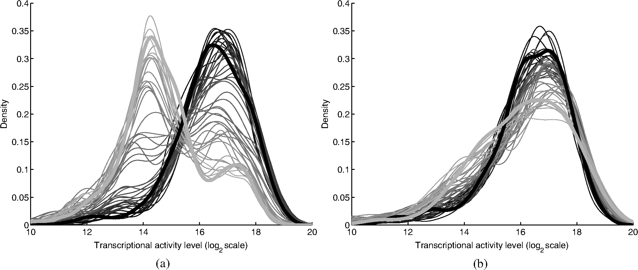 The control population shows that without the influence of the drug, the transcription activities remain high in most of cells and only start to decrease in a small portion of cells at the end of the experiment, probably due to the depletion of growth factors in the media. This also confirms that there is little photobleaching in unaffected cells. More revealingly, the bi-modal expression profiles demonstrate beyond any doubt that when turning off, the state transition of MKI68 transcription activity is more of a switch-like procedure, rather than a gradual decrease of transcription level over the whole cell population. Furthermore, the switch-off of the transcription activity among responsive cells is not well synchronized, indicating different latency periods for cells to responding to the drug or even the existence of resistant sub-populations in the cell culture. Such a response dynamic is only observable when individual cell transcription activities, rather than the overall activity, are identifiable. Viewing expression profiles as density functions allows researchers to compare transcription activities under different conditions in a single plot. In Fig. 5, the transcription activities at different time points are compared. One can also compare the transcription activities under multiple conditions, such as different drugs or cell-lines. One can also put different plots side-by-side and make larger-scale comparisons. While providing a means for direct comparison, a density function does not quantify observed differences. Thus, while this density-based approach can provide straightforward comparison for small-scale studies, where only a few factors are involved and there are few conditions to track and compare, it is less suitable for studies of complex diseases like cancer, where one would like to perturb the cell-line of interest with multiple drugs aiming at different targets and track multiple transcription signatures representing several critically related pathways. To represent the cellular activities at such a large scale in a manageable manner, one needs to further quantify the expression profile while keeping the meaningful responses observable. From the example shown Fig. 5 as well as other observations, we notice that, for a cell culture at any given time, the distribution of transcription activity is mostly either uni-modal or bi-modal, indicating the cells are in either one or two dominating states most of the time. In the beginning of the experiment, owing to careful preparation, the transcription activity is highly homogeneous and the density function is always uni-modal with a sharp peak. Moreover, when the cell culture reacts to certain stimuli, the response is mostly uni-directional, which can lead to bi-modal distribution during state transition. If one could identify the valid states which the transcription activity can occupy and the percentage of cells in those states for any give time point, then the most informative part of the cellular dynamical system could be captured. However, we have found that such an absolute measure of cellular response is not practical on account of the following reasons: (1) It is hard to determine whether the distribution is uni-modal or bi-modal in many cases, especially when the estimated density functions is not smooth or during the transient period when cell response commences but is not prominent. (2) Assuming the nature of the distribution is correctly identified, then in a bi-modal case, if the two peaks are too close or the minor peak is too small, the state position of the minor peak could be hard to identify. (3) The absolute values of the transcription activity of the case population are of little meaning unless they are benchmarked against a control population. To ensure robustness of the quantified results, rather than using absolute measures, we adopt a relative measure that quantifies the transcription activity changes with respect to a control population. As a relative measure, our quantification procedure intends to determine the size of the case population that behaves differently from the control population and the magnitude of the difference, which we denoted as pop-shift (PS) and fold-change (FC), respectively. We denote the distributions of the case and control populations as and , respectively, and their corresponding density functions as and , respectively. The control population can represent any condition that makes the comparison meaningful. The most common choice is the unperturbed population at the same time point, although it is also common to choose the same population at the beginning of the experiment. The intuitive idea for PS and FC is shown in Fig. 6. Basically PS measures the non-overlapped areas of the two distributions, as indicated by either grey area in Fig. 6, left and right representing the difference between and where and where , respectively. Because and are density functions, the two grey areas are of same size, i.e., Note that PS can be conveniently computed by using the total variation distance.26 Fig. 6Quantification of the relative transcription level shift and the percent of the population of cells showing altered transcription levels are carried out as shown to produce pop-shift and fold-change estimates.  For two identical distributions, , while for two totally disjoint distributions, . To evaluate FC, we measure the distance between the mass centers of the two non-overlapped areas, which indicate the extent of the population shifts: Note that the FC can be conveniently computed as, which is essentially the distance between the means of the two distributions, normalized by PS. Fold-change can be either positive or negative, indicating whether the transcription activity is increasing or decreasing with respect to the reference case.The product of PS and FC is given by the difference of mean cell-expression levels, Although, average expression levels or similar ideas are commonplace in many high-throughput genomic data collection techniques, such as microarrays, the term used here is actually different. The critical difference is that the average here is taken at the cell level over the log-transformed values, whereas the microarray expression level is averaged in the assay during sample preparation and the log transform is taken after the average expression level is retrieved. Thus, the measure used here can improve detection sensitivity by mitigating the distorting impact of over-expressing outliers, which can have concentration levels hundreds of times higher than most of the other cells. The PS and FC measures assume case population shift in one direction with respect to the control population and are most reliable when the assumption holds. There are cases this assumption is violated. The most common case is when the majority of the cells are shifting towards one direction but there can be a small number of cells shifting in the opposite direction. For example, in the beginning of the experiment, the cell culture is prepared so that the cells are in a quite homogeneous state. However during the on-going experiment, the cells begin to show increased variance in activity even without any external stimulus. The increased variance can be detected as cells shifting to both directions, although there is no meaningful state change. Such a behavior uncertainty could be even higher if the cells are under perturbation. In such cases, PS will report the total cells shifting to both directions while FC will report only small change. The measures hence could be misleading when there is only a small population shift, and affect the detection of the response initiation, which is critical to identifying the order of events. To alleviate this problem, we introduced a modified measure pair by computing both the up-regulation and down-regulation changes. Letting the up- and down-regulated PS and FC can be computed separately based on the distribution is to the left or right of :indicates that any shift to the left is down-regulation, whereas indicates up-regulation. The relationship between the bi-directional PS and FC to the uni-directional pair is straightforward: Since we assume the state shift is uni-directional, any shift to the opposite direction is only due to noise or some transient activity. Hence, it is worthwhile to combine the measures into one pair according to the following procedure by canceling out the shifts to both directions. We first determine the dominating shifting direction based on and then compute the modified values: The modified fold change is the FC of the dominating direction, while the modified pop-shift is based on the mean cell-expression level difference and . Rather than cancelling out the PS directly, we choose to use the mean cell-expression level to cancel out the product of PS and FC. This is because the noisy PS terms are usually a slight shift with relatively large PS but small FC. In comparison, a true shift is normally initiated with a far greater FC level but a relatively small percentage of cells. Thus, using the mean cell-expression value can help us identify the initiation of a true state transition. An alternative choice is to use the PS and FC of the dominating direction without canceling out any shift; however, we have noticed that if the PS in the opposite direction is due to noise, say variance, then it usually affects both directions, although the one in the dominating direction is over-shadowed by the true transition and therefore is not detectable. Once the PS and FC values are calculated for all time points of a certain condition, the PS and FC time sequences are separately smoothed with a median filter to remove small irregularities. To show the transcription activity changes summarized by the PS and FC pair, we use a bar-plot pair as shown in Fig. 7, which refers to the same drugged cell population imaged and processed in Figs. 1 and 5(a). In Fig. 7(a), the initial state of the drugged population was chosen as the control, so for each time point, its current expression profile was compared to its own expression profile at the beginning of the experiment to obtain the PS and FC pair. In Fig. 7(b) the un-drugged population shown in Fig. 5(b) was chosen as the control, so for each time point, drugged population’s current expression profile was compared to the expression profile of the same time point of the control population. In each plot, two bar-plots are put in parallel pairs with common -axis aligned with experiment time points. The top bar-plot represents PS, while the bottom bar-plot, which is drawn downwardly, represents FC. In order to make the whole plot compact for better comparison, the absolute value of the change is shown and different fillings are used to indicate up- or down-regulation: white for increased activity and black for reduced activity. Each tick in the -axis of the PS plots corresponds to a 10% shift. The -axis for FC plots is shown in scale, i.e., two consecutive ticks indicate a twofold difference in concentration. Finally, although the PS and FC pair can reveal most of the cellular response activities, sometimes it’s still helpful to have a measure on the absolute expression levels. Here we chose the initial state, represented by the peak positions in the density functions at the beginning of the experiment, to provide a general idea on the absolute transcriptional level of the target gene. The initial states of both case and control populations are shown at the left of the plot. Fig. 7The bar-plots show the relative transcription activity of the cell population of Fig. 1 throughout the experiment with the control population set to: (a) the initial population distribution at the beginning of the experiment; (b) the untreated population at the same time point. The drug was added after 5th hour. The top bar-plots show the pop-shift, while the bottom ones show the fold-change. Each tick upward on the -axis of the upper, population-shift plots corresponds to 10% shift in population, while each tick downward on the -axis of the lower, fold-change, plots indicate a 2-fold difference in expression level. The white bars indicate up-regulation while the black bars indicate down-regulation. The expression levels of the initial state for both case and control are shown at the left of each plot as the of the green fluorescent intensity.  Figure 7 shows that under the influence of the drug lapatinib, the transcription of gene MKI67 is turned off, starting from about 10 to 15 h after the drug is added. At the end of the experiment, transcription activities of about 40% of the cells have decreased to to of the no-drug control activity level. 3.Results and DiscussionTo validate use of the proposed data analysis procedure, we have conducted comprehensive experiments to evaluate performance. 3.1.Image Processing PerformanceThe essential performance measure for image processing is nuclei segmentation accuracy. To evaluate nuclei segmentation accuracy, we have randomly selected 4 fluorescent images from 4 different imaging sites that cover over 1000 nuclei. Besides the proposed method, two other methods are used: segmentation by the software CellProfiler27,28 and manual segmentation. CellProfiler is a free open-source cell image analysis software developed by the Broad Institute. We have used Cell Profiler 2.0 (r10997). The nuclei segmentation is conducted through the module Identify Primary Objects, which uses a thresholding-based approach followed by shape-based de-clumping. Since the size of the foreground region in our cell image can vary substantially from image to image and from time to time, based on the suggestions from the software, we choose the two-class Ostu Adaptive segmentation as the thresholding method. The default threshold is too lenient for the cell density observed in our experiment, thus a threshold correction factor of 10 is set to achieve good segmentation of the selected images. For the proposed method, no specific individual parameters are selected for the four images; instead, we used a global parameter setting, which is actually used for all images processed in this paper. Since there is no ground truth for the segmentation, we use manual segmentation by M. L. Bittner, one of the co-authors, who has three decades experience with cell and nuclear morphology, as a benchmark and compare the other approaches to this manual benchmark for accuracy counts. We also consider another independent manual setting by another experienced biologist. The inconsistency between the manual segmentations provides an idea of how well one could hope to do in comparison to the chosen standard. If two experienced biologists can only agree on 90% of the segmentation results, then it is likely that any claim of above 90% for automatic segmentation is just accidental. Accuracy counts are divided into three categories: consistent nuclei, under-/over-segmentation, and missed nuclei. Segmentation results are shown in Table 1(a). Performance is comparable for CellProfiler and the proposed method at about 85% accuracy rate. CellProfiler’s performance decreases slightly when the cell density is high or the number of cells is large (over 300). Although the manual segmentation performance is better (relative to the benchmark manual segmentation), it is still below 90% and only 4% better than automatic segmentation methods, reflecting the overall difficulty of the problem and indicating good performance for the automatic methods. It should be noted that the total number of nuclei identified by each method are not the same. For computer-based approach, the most common errors are the over- and under-segmentation, while for manual segmentation, the discrepancy on whether to identify a certain object as cell play a much larger role in accuracy rate. Table 1Accuracy of nuclei segmentation: (a) 4 random selected images from 4 different sites; (b) an image later in the experiment from a site used in (a).
To check the robustness of the image processing, we examine images of the same sites of the four images evaluated in Table 1(a) but at different time points of the experiment. In general, both automatic segmentation methods work pretty well, except for one site, where the nuclei intensity has dropped significantly at the later stage of the experiment. To illuminate the problem, another sample image of that site has been picked out for accuracy counting and the results are listed in Table 1(b), where we see that the segmentation performance has decreased significantly for all methods, with CellProfiler at a paltry 39.3%. The proposed method’s performance at 69% is even better than the manual segmentation, reflecting the great uncertainty even for the experienced biologists. This large discrepancy is due to the extreme condition experienced by the cells under great pressure. Although the dye on the nuclei has become dimmer, the chromosomes have begun to shrink into small yet bright nodes, making it much harder to tell whether an object contains single or multiple nuclei. Moreover, some nuclei have started to break up, a sign of apoptosis, thereby creating small particles that further confuse the segmentation procedure. Overall, the proposed image processing protocol can provide fast and robust image segmentation performance with adequate accuracy for the purpose of the experiment. We didn’t use CellProfiler not due to its general performance, but because of its lack of robustness relative to the kind of image degradation that can occur with our technology—for normal images, both CellProfiler and our approach provide segmentation accuracy close to human performance. 3.2.ReproducibilityTo compare gene expression profiles obtained under the same condition and derive an empirical distribution of profile difference under the identical condition, we measure the variability of duplicated cases. If the experiment and data analysis protocol are highly reproducible, then there should be little difference. In one experiment, we have collected 56 wells of identical condition: cell-line HCT116, reporter for gene MKI67, with no drug applied. Each well contains one imaging site. The experiment lasts 48 h, with images taken at every hour. After image processing and quality check, three time points were removed due to low imaging quality in significant number of imaging sites. The results of the remaining 45 time points are used to compute the profile difference distribution by emulating the standard experimental design, where each condition is covered by three sites. A scheme based on random sampling is used:
Thus by aggregating all PS values, we have an empirical distribution for profile variation of identical condition based on PS, which is equivalent to total variation, an important distance measure for probability distributions.26 Figure 8(a) shows the distribution of PS values over all time points. For most case pairs, the reproducibility is very high, with PS values between 0.03 and 0.06, and very few PS values over 0.1. Additionally, the empirical distribution of Fig. 8(a) can help researchers identify genuine response differences. Taking identical condition as null hypothesis, the empirical distribution in Fig. 8(a) indicates that a PS value over 0.072 will lead to the rejection of the null hypothesis at significance level 0.05, and a threshold of 0.09 corresponds to the significance level 0.01. Thus if the PS value between the expression profiles of target case and control case is larger than 0.1, one can confidently claim there is a significant difference in the transcriptional response that is worth further investigation. Figure 8(b) shows the thresholds at significance level of 0.05 and 0.01 for each time point, based on the empirical expression distribution of that time point. It can be seen that there is little change in the thresholds at different time points, indicating that the reproducibility is not significantly affected by the time factor for at least 48 h. Fig. 8(a) The empirical distribution of PS between cases of identical condition is shown. (b) The thresholds of population shift corresponding to significance levels at 0.05 and 0.01 are shown for all time points. 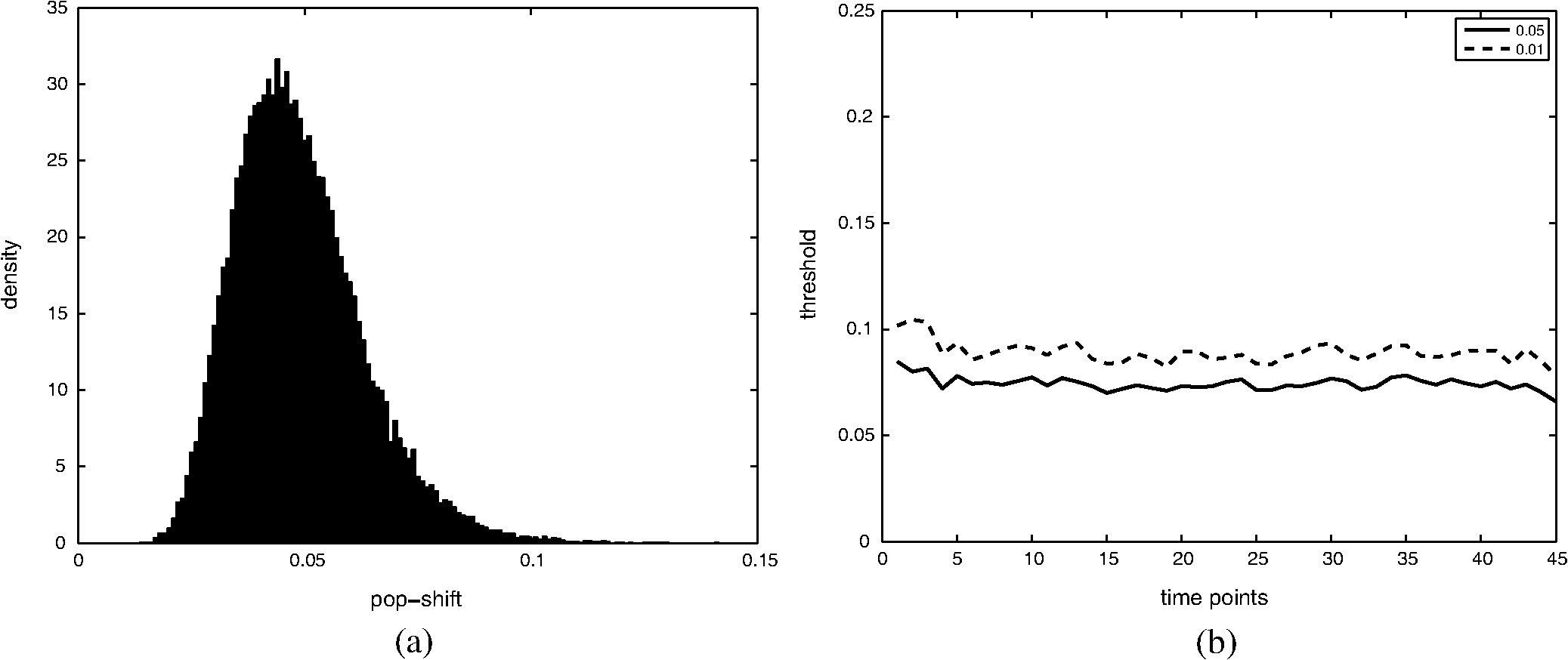 Finally, we should point out that the empirical distribution obtained in Fig 8(a) is based on duplicated sites in one plate. Our experience shows that certain experimental factors, like how the sample is prepared, can have direct effects on the outcome, mostly shifts in the expression distribution and/or response dynamics. Thus to ensure reliable comparison, one should carefully prepare the assay so all conditions for direct comparison are in one plate, or in plates that are prepared and imaged as one batch. The tight confidence interval and time-invariance between duplicated cases confirm that the proposed image and data analysis protocol can provide reliable, robust and consistent performance for properly designed experiments. 3.3.SensitivityTo evaluate the proposed protocol’s ability to discriminate slight differences in a set of responses, we have designed an experiment where different drug doses are applied to incur different responses. Again, the cell-line HCT116 and the reporter for gene MKI67 are picked. As seen from Fig. 7, HCT116 is sensitive to the drug lapatinib and the transcription of MKI67 will be turned off when the drug is properly applied. In our experiment, six different doses of lapatinib, varying from a very light dose of 1 micromolar (µM) to a higher-than-normal dose of 32 µM are applied to the HCT116 cell-line after the fifth hour and the experiment lasts a total of 48 h. Six duplicates are used to cover each condition. The bar plots in Fig. 9 show the extracted transcription responses to the drug. To facilitate unbiased evaluation, all corresponding axes across the plots are of the same scale. Since all cases share the same control population, the initial states of all six controls are of the same value. The initial states of all cases are very close to the control state, indicating that the samples are well prepared for the experiment. The effects of different dosing amounts can be clearly seen through direct comparison of the bar-plots. The response magnitudes induced by the drug increase consistently with the dosing amount. The smaller dosing amounts of 1 and 2 µM have observable yet small responses. The 8 µM dose was used in many experiments and has been shown to produce 50% growth inhibition in this cell line. In our experiment, this dose induces a considerable response, and the shift of cells to the reduced expression population is still rising at the end of the experiment. The highest dosing amounts of 16 and 32 µM induce the largest pop-shifts and show signs of saturation at the end of the experiment. Another sign of possible saturation is the relatively smaller extent of fold-change in the highest doses. The difference in the time when responses are initiated can also be readily observed, with the highest doses showing clear responses at five to 10 h after the drug, followed by normal doses at around 15 h, and lowest doses at even later hours. The dose response experiment clearly shows that the proposed protocol is sufficiently sensitive to detect small differences in transcriptional activities. Fig. 9Bar-plots of dose response results produced by different drug dosages. The bar-plots are ordered by dosing level, as indicated at the right side of the plots.  It is interesting to note that for the response of the lowest dose, if observed alone, its PS values are never high enough to register as a significant response; however, if compared with other cases of related yet non-identical conditions, as the cases shown in Fig. 9, the similarity between this case and other responses can hardly be missed and its contribution to infer the underlying biological mechanism can be rightfully appreciated. Thus, the power of the proposed protocol to detect mechanisms responding to certain perturbation can be further boosted through properly designed experiments. 3.4.Full-Scale ExampleIn previous experiments, we have focused on evaluating specific qualities of the proposed protocol. As a high-content analysis tool, we expect the data analysis should allow researchers to not only follow the transcriptional activities of multiple genes simultaneously but also be able to compare these cellular activities side-by-side for different conditions. In this section, we discuss a full-scale experiment to demonstrate the ability of the data analysis protocol to cover cell process dynamics and reveal hard-to-detect relationships between responses induced by different conditions. We have further screened the colon cancer cell line HCT116 against a variety of drugs. A total of 17 reporters have been selected to cover the genes for proliferation and survival pathways, two vital pathways in a cancer cell-line, and some other related genes. Figure 10 shows the diagram of two pathways, proliferation on the left and survival on the right. The wiring scheme has been greatly simplified to keep only key components in the diagram. It should be noted that this diagram is based on common knowledge of the two pathways and is not necessarily an accurate description of the cell-line under study. The genes for which reporters are used to assess their transcription are marked by shaded boxes. The drugs used in the experiment are marked in bold text. Fig. 10A simplified wiring diagram shows the key components of proliferation (left) and survival (right) pathways, and other related genes. The genes whose transcriptional activities can be assessed through a reporter are marked by shaded boxes. The drugs are labeled in bold text. 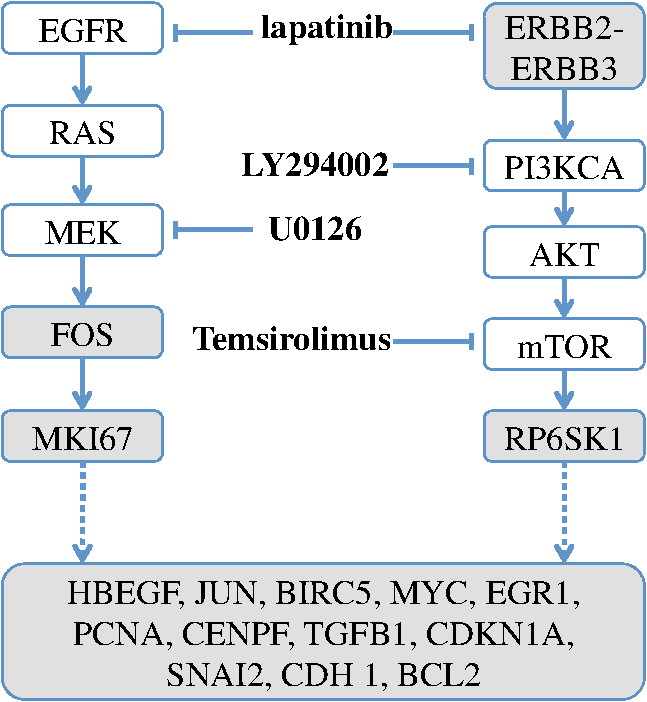 Figure 11 shows the bar-plots for the transcriptional responses of all 4 drugs. Each column corresponds to a drug, while each row corresponds to a gene reporter, with the gene name associated with the reporter shown at the right end of that row. Because the experiment is conducted with multiple plates in several runs, whose duration time is different from each other due to various causes, the bar-plots are of different length. To ensure reliable comparison, all conditions associated with the same gene reporter, including the control populations, are contained in the same plate, and thus have been imaged in the same run. The same scale is set to the corresponding axes in all plots to facilitate accurate comparison. Fig. 11The bar-plots of relative transcriptional activity in HCT116 for four different drugs are presented.  From the bar-plots one can see that all four drugs induce some levels of responses. By showing all reporter responses in one large plot, the patterns in drug response can be more easily detected. Lapatinib induces responses of largest scale, with all but one reporter showing a clear decrease in transcription activity. Specifically, reporters of MYC are down-regulated only in a small portion of cells at the end of the experiment, but in terms of the full transcription profile, it is highly possible that this small shift is no accident. The behavior is consistent with the knowledge in the wiring diagram where lapatinib can inhibit both EGFR in the proliferation pathway and the ERBB2/3 heterodimer in the survival pathway. In comparison, U0126 only induces strong responses in a limited number of reporters, for instance, EGR1, FOS, and MKI67. For the reporters responding with down-regulation, the fold-change is relatively small compared to other drugs that induce similar pop-shifts, and most of these genes are closely related to the proliferation pathway. All of these observations are consistent with knowledge that U0126 is only targeted to a downstream member of the proliferation pathway and the observations confirm the limited scope of U0126’s impact. In comparison, LY 294002 induces a response pattern similar to lapatinib but of smaller degree in HCT116, which is consistent with the fact that LY 294002 targets only the survival pathway. The most revealing case is Temsirolimus, which exemplifies how the transcription activity bar-plots can uncover subtle and hard-to-discover relationships. Under initial examination, the responses to Temsirolimus are so small that one is likely ignore them if any single reporter is examined alone; however, since all 17 reporters are shown in one plot and 12 of them end at down-regulation states, one is led to consider the overall response pattern. A close examination of the response pattern of LY 294002 shows that out of 17 reporters, 15 are at down-regulation states at the end of the experiment and the two in up-regulation, CDKN1A and MYC, are also up-regulated for Temsirolimus. This similarity reveals that Temsirolimus and LY 294002 are probably targeting the same pathway, but with different drug efficiency. This hypothesis is confirmed through the wiring diagram in Fig. 10, where Temsirolimus targets mTOR, a gene downstream of LY 294002’s target gene PI3KCA. These kinds of observations lead one to reasonably believe that, with careful design, similar procedures can be used to explore relationships between other drug pairs, including compounds of unknown mechanism. 4.ConclusionHigh-content fluorescent protein reporter imaging can be used to track transcriptional activities in parallel. The huge amount of data collected from such an imaging protocol calls for innovative ways to analyze the data. In this paper, we introduced a data processing procedure to extract cell processing dynamics in a reliable and timely manner. The procedure contains two parts: (1) image processing, where the fluorescent images are processed and the transcriptional levels are extracted and quantified; and (2) data representation, where the extracted data are summarized into expression profiles and the transcriptional responses are transformed into informative bar-plots to facilitate efficient evaluation. The proposed data processing procedure provides a systematic solution for examining the experiments at different abstraction levels. Researchers can have a general idea of the whole experiment with bar-plots and further examine the details with expression profiles, or the raw images, if needed. Our experiments showed that the proposed procedure can achieve fast and robust image segmentation with adequate accuracy. The results are highly reproducible, and sensitive enough to detect subtle differences and hidden relationships. The method can help biologists take the advantage of high-content screening technology, accelerate identification of mechanisms underlying potential drug candidates, and in general increase the efficiency of drug discovery and treatment design. Notes*In such case, before the main part of the image processing starts, the reference sites are pre-processed to extract the background intensity and saved in a common file. During the image segmentation, the background will be loaded from the common file, rather than processing the reference sites. †Imaging a 384-well plate requires approximately 43 min when using two color channels and taking two images per well, leaving only a small amount of free time to process images. Like most commercial automated epifluorescence image-acquisition systems, the authors’ systems do not provide simultaneous image capture and image-analysis support. ‡Although in this study images were taken by IN Cell Analyzer 3000, the general cell-handling and imaging protocol works reliably on another commonly used robotic imager (Molecular Devices, ImageXpress Micro) which has similar autofocus control, a single cooled CCD camera and a Xenon flashlamp excitation source. AppendicesAppendix:A1.Biological Sample PreparationIf a report of the promoter activity level of a specific gene is desired, then a DNA segment of that promoter ( to 2000 base pairs) upstream of the start of transcription for the gene of interest is copied using PCR and cloned into a plasmid pENTR5′ (Life Technologies, K59120), where it is flanked by recombination sites. Such a promoter donor plasmid along with another donor plasmid pENTR11 (A10467) with an eGFP protein coding sequence flanked by recombination sites are used to deliver the promoter and coding sequence via recombination into a recipient lentiviral delivery vector pLenti6.4/R4R2/V5-DEST (A11145) to create a cassette where the promoter of interest will drive the production of eGFP mRNA, which will be translated into fluorescent protein. The lentiviral vector can be transfected into 293FT cells along with helper plasmids that allow RNA copies of the cassette to be produced and encapsulated into particles that are readily taken up by cells, converted into a DNA copy, and integrated into the genome of the that cell, so that the promoter reporter construct resides stably in that cell. In order to maximize the uniformity of reporter signaling in the population of cells carrying the reporter construct, it is useful to introduce the expression cassette in a uniform way. The lentiviral delivery system allows delivery of cassettes containing the promoter/reporter and blasticidin drug resistant portion of the initial construct in a dose-dependent fashion. These particles can effectively transduce both dividing and non-dividing mammalian cells with the promoter/reporter construct. Cells to receive the reporter are infected at a multiplicity of infection of 0.5 to 0.7, which limits the delivery to one construct per cell to nearly all of the cells that do get infected. The cells are then cultured for three days in the presence of blasticidin, which kills those cells that were not infected, at which point, the cells are ready for use in the assay. Response dynamics experiments are carried out to determine whether or not a particular drug perturbs a set of processes hypothesized to be altered by the drug. To test the hypothesis, a set of reporters that each evaluates the process activity level at a particular point in the process is required. To allow testing over a wide variety of cellular processes, we have built a GFP library containing over 80 GFP reporters that cover known critical cellular responses. A set of 17 GFP reporters for analysis of proliferation and survival activities in cell line HCT 116 (ATCC #CCL-247) are utilized in this study. HCT 116 reporter-bearing derivative cultures are cultured in DMEM (Life Technologies, 11965118), supplemented with 10% FBS (16000044), 20 mM Hepes (15630080), 20 mM Glutamax (35050061) and 1% Penicillin—Streptomycin (15070963) in T25 flasks. For imaging, a media having low levels of autofluorescence, IM, is prepared. IM contains 70% M-199 (11825015), 30% RPMI-1640 (11875085) supplemented with 10% FBS (16000044), 20 mM Hepes (15630080), 20 mM Glutamax (35050061) and 1% Penicillin—Streptomycin (15070963) and 0.5 µM Vybrant® DyeCycle™ Violet Stain (V35003). The stain is live-cell permeable and produces blue fluorescence () when bound to double-stranded DNA and stimulated with a violet excitation source (). One day prior to an imaging experiment, sub-confluent cells are trypsinized to release them from the flask surface, resuspended in IM and counted in an automated cell counter (Life Technologies C10227) to establish number of cells per milliliter. The concentration of cells is then adjusted to 1500 cells per 30 µl of IM. A 30 µl aliquot of cells having a particular promoter/reporter construct is delivered to a well in a 384-well microtiter plate (Greiner Bio-One 781 09x) that has black, opaque walls and a thin, UV-transparent well-bottom. The plate wells were previously collagen coated by exposing them to Rat Tail Collagen Type I (BD Biosciences 354249) in 0.02 M acetic acid for 1 to 4 h followed by washing 2 times with 1× PBS (Gibco 14200). The cells were allowed to attach to the plate and equilibrate for 14 to 16 h in a tissue culture chamber prior to beginning imaging. Each condition tested used six replicate wells in reproducibility and sensitivity experiments, and three replicate wells in the full-scale example. A2.ImagingAll images examined in this study were taken by an automated scanner (IN Cell Analyzer 3000, General Electric) with a objective.‡ Images were captured using three high-speed cooled CCD cameras for Blue, Green and Red fluorescent channels. Excitation was provided by three separate lasers. Throughout the experiments the focus of the scanner was automatically adjusted using an infrared laser to determine the liquid/well bottom interface and then applying a defined offset per channel. Flat-field correction was determined by imaging wells with slightly fluorescent media prior to the start of the experiment. While imaging, the humidity in the imaging chamber holding the plate is controlled at 70%. The level is controlled at 5% by mixing with ambient air at the proper ratio. The gas mixture is then pumped through a heating and moisturizing chamber to bring it to 37°C. Then the experiment plate was imaged continuously once per hour for 5 h to obtain baseline data. Another 30 µl aliquot of IM was then added which contained perturbants at twice the concentration desired or no additives for control wells and again imaged once per hour for the duration of the whole experiment, which usually lasted up to about 48 h under our experimental settings. After the imaging, the flat-field-corrected images were exported in uncompressed tiff format for image analysis. AcknowledgmentsDevelopment of these methods was supported in part by a contract from PBS-Bio and a generous grant from the W.M. Keck Foundation. ReferencesM. Chalfieet al.,
“Green fluorescent protein as a marker for gene expression,”
Science, 263
(5148), 802
–805
(1994). http://dx.doi.org/10.1126/science.8303295 SCIEAS 0036-8075 Google Scholar
L. Haoet al.,
“Comprehensive analysis of gene expression patterns of hedgehog-related genes,”
BMC Genomics, 7 280
(2006). http://dx.doi.org/10.1186/1471-2164-7-280 BGMEET 1471-2164 Google Scholar
T. KandaK. F. SullivanG. M. Wahl,
“Histone-GFP fusion protein enables sensitive analysis of chromosome dynamics in living mammalian cells,”
Curr. Biol., 8
(7), 377
–385
(1998). http://dx.doi.org/10.1016/S0960-9822(98)70156-3 CUBLE2 0960-9822 Google Scholar
R. PepperkokJ. Ellenberg,
“High-throughput fluorescence microscopy for systems biology,”
Nat. Rev. Mol. Cell. Biol., 7
(9), 690
–696
(2006). http://dx.doi.org/10.1038/nrm1979 NRMCBP 1471-0072 Google Scholar
S. A. Haney, High Content Screening: Science, Techniques and Applications, Wiley-Interscience, Hoboken, N. J.
(2008). Google Scholar
A. H. GoughP. A. Johnston,
“Requirements, features, and performance of high content screening platforms,”
Meth. Mol. Biol., 356
(11), 41
–61
(2006). http://dx.doi.org/10.1385/1-59745-217-3:41 MMBYBO 0097-0816 Google Scholar
X. Zhouet al.,
“Towards automated cellular image segmentation for RNAi genome-wide screening,”
885
–892
(2005). Google Scholar
B. Neumannet al.,
“High-throughput RNAi screening by time-lapse imaging of live human cells,”
Nat. Methods, 3
(5), 385
–390
(2006). http://dx.doi.org/10.1038/nmeth876 NMAEA3 1548-7091 Google Scholar
K. KornE. Krausz,
“Cell-based high-content screening of small-molecule libraries,”
Curr. Opin. Chem. Biol., 11
(5), 503
–510
(2007). http://dx.doi.org/10.1016/j.cbpa.2007.08.030 COCBF4 1367-5931 Google Scholar
N. HarderR. EilsK. Rohr,
“Automated classification of mitotic phenotypes of human cells using fluorescent proteins,”
Meth. Cell Biol., 85 539
–554
(2008). http://dx.doi.org/10.1016/S0091-679X(08)85023-6 MCBLAG 0091-679X Google Scholar
F. Liet al.,
“Workflow and methods of high-content time-lapse analysis for quantifying intracellular calcium signals,”
Neuroinformatics, 6
(2), 97
–108
(2008). http://dx.doi.org/10.1007/s12021-008-9016-z 1539-2791 Google Scholar
F. Spyratoset al.,
“Correlation between MIB-1 and other proliferation markers: clinical implications of the MIB-1 cutoff value,”
Cancer, 94
(8), 2151
–2159
(2002). http://dx.doi.org/10.1002/(ISSN)1097-0142 CANCAR 1097-0142 Google Scholar
F. FanK. V. Wood,
“Bioluminescent assays for high-throughput screening,”
Assay Drug Dev. Technol., 5
(1), 127
–136
(2007). http://dx.doi.org/10.1089/adt.2006.053 ADDTAR 1540-658X Google Scholar
D. HanahanR. A. Weinberg,
“Hallmarks of Cancer: The Next Generation,”
Cell, 144
(5), 646
–674
(2011). http://dx.doi.org/10.1016/j.cell.2011.02.013 CELLB5 0092-8674 Google Scholar
E. R. DoughertyR. A. Lotufo, Hands-on Morphological Image Processing, SPIE Optical Engineering Press, Bellingham, Washington
(2003). Google Scholar
S. OsherN. Paragios, Geometric Level Set Methods in Imaging, Vision, and Graphics, Springer, New York
(2003). Google Scholar
A. Dufouret al.,
“Segmenting and tracking fluorescent cells in dynamic 3-D microscopy with coupled active surfaces.,”
IEEE Trans. Image Process., 14
(9), 1396
–1410
(2005). http://dx.doi.org/10.1109/TIP.2005.852790 0278-0062 Google Scholar
P. Yanet al.,
“Automatic segmentation of high-throughput RNAi fluorescent cellular images.,”
IEEE Trans. Inf. Technol. Biomed., 12
(1), 109
–117
(2008). http://dx.doi.org/10.1109/TITB.2007.898006 1089-7771 Google Scholar
L. VincentP. Soille,
“Watersheds in digital spaces: an efficient algorithm based on immersion simulations,”
IEEE Trans. Pattern Anal., 13
(6), 583
–598
(1991). http://dx.doi.org/10.1109/34.87344 Google Scholar
L. Vincent,
“Grayscale Area Opening and Closing, their efficient implementation and applications,”
Proc. Eurasip Workshop on Mathematical Morphology and its Applications to Signal Processing, Barcelona, Spain(1993). Google Scholar
R. A. Weinberg, The Biology of Cancer, 22
–27 Garland Science, UPC PublicationsNew York
(2007). Google Scholar
E. Parzen,
“On the estimation of a probability density and mode,”
Ann. Math Stat., 33
(3), 1065
–1076
(1962). Google Scholar
A. W. BowmanA. Azzalini, Applied Smoothing Techniques for Data Analysis: The Kernel Approach with S-Plus Illustrations, Clarendon Press, Oxford
(1997). Google Scholar
S. J. SheatherM. C. Jones,
“A reliable data-based bandwidth selection method for Kernel density estimation,”
J. Roy. Stat. Soc. B: Met., 53
(3), 683
–690
(1991). 0035-9246 Google Scholar
J. S. Marron,
“Smoothing, Functional Data Analysis, and Distance Weighted Discrimination Software,”
(2004) http://www.unc.edu/~marron/marron_software.html Google Scholar
L. DevroyeL. GyörfiG. Lugosi, A Probabilistic Theory of Pattern Recognition, Springer-Verlag, New York
(1996). Google Scholar
A. E. Carpenteret al.,
“CellProfiler: image analysis software for identifying and quantifying cell phenotypes,”
Genome Biol., 7
(10), R100
(2006). http://dx.doi.org/10.1186/gb-2006-7-10-r100 GNBLFW 1465-6906 Google Scholar
M. R. LamprechtD. M. SabatiniA. E. Carpenter,
“CellProfiler: free, versatile software for automated biological image analysis,”
Biotechniques, 42
(1), 71
–75
(2007). http://dx.doi.org/10.2144/000112257 BTNQDO 0736-6205 Google Scholar
|
|||||||||||||||||||||||||||||||||||||||||||||